Cellular Automata

The term cellular automata (singular: cellular automaton) refers to a class of simple computational models. A cellular automaton consists of a set of cells that we usually think of as being arranged in some repeating geometric pattern. For example, cells might consist of individual square boxes in a line, or a grid of squares in the plane, though the same ideas can be applied to more exotic arrangements of cells. Each cell has cells which are said to be neighbors or adjacent cells. When defining a cellular automaton, one must specify the way in which adjacency is determined. Together, the set of cells and their neighbors determine the automaton’s network structure.

The following image depicts a one dimensional grid network structure. We’ve highlighted one cell, while its two neighboring cells are filled in gray.

This image depcits a two dimensional grid network structure. For a two dimensional grid, there are two natural choices of neighbors for each cell. One is that the neighbors of each cell are the four cells with wich the cell shares a side (depicted in dark gray below). Another option would be for each cell to have eight neighbors as depcited in both light and dark gray below.

A description of a cellular automaton also includes a set of states that each cell can attain. Typically, there is a fixed (small) number of possible states for each cell. In this note, we will focus on the case where there are only two possible states for each cell: 1 and 0. An assignment of states to each cell in the network is referred to as a configuration.

Here is an example configuration of a one dimensional grid where the 1 states are filled in black, while the 0 states are indicated in white.

Similarly, here is a configuration of a two dimensional grid network.

The states of a cellular automaton evolve according to a rule a.k.a. transition function that determines how each cell should update its state. The rule specifies how each cell should update its state based only on its current state and the state of its neighboring cells. All cells update according to the same rule, but different cells will generally adopt different configurations depending on the states of their neighbors. We refer to a single update of all cells in the network a step. An execution of a cellular automaton is the sequence of configurations obtained by repeatedly applying the update rule to all cells in the network.

Example. The following figure illustrates an execution of a 1D cellular automaton with the following update rule: a cell adopts the state 1 if either neighbor is in state 1, and adopts the state 0 otherwise. We use the initial configuration consisting of a single central cell in state 1, while the other cells are in state 0. Each row in the figure depicts a single step in the execution of the automaton. We refer this figure as the space-time diagram of the execution: the horizontal axis represents space (i.e., the cells in the network), while the vertical axis represents time (measured in steps of the execution). Thus, the top row is the initial configuration. The second row is the state after one update step, and so on.

One-Dimension, Two States

For the remainder of this note, we will consider one-dimensional (1D), 2-state cellular automata. That is, the network consists of a one-dimensional array of cells, and each cell can be in one of two states, 0 or 1. We assume that the array is a circular array: the right neighbor of the right-most cell is the left-most cell and vice versa. This way, every cell has exactly two neighbors: one left, and one right. (An alternative convention that we will not use is that the array extends infinitely in both directions.)

For 1D 2-state automata, an update rule for the cells must depend only on the current states of (1) the cell, (2) the cell’s left neighbor, (3) and the cell’s right neighbor. Since there are only 2 options for each of these states, a rule is completely determined by \(8 = 2^3\) values. We can represent a rule by specifying how the cell should update its state in the eight possible scenarios. Here is a visual depiction of such a rule:

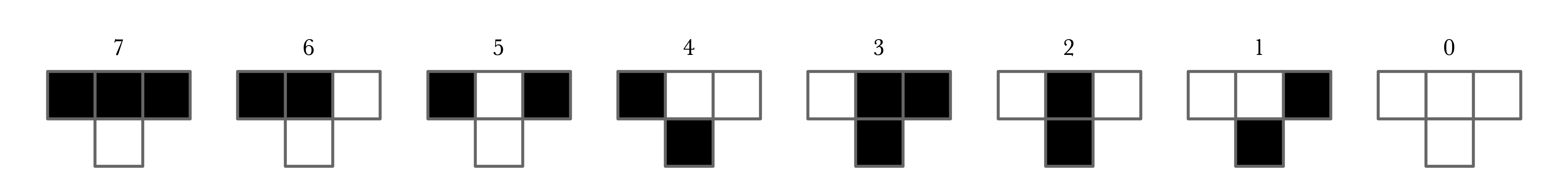
For example, the right-most figure indicates that if a cell and both of its neighbors are all in state 0, then the cell’s next state will be 0. The next figure from the right indicates that if the cell and its left neighbor are in state 0 and the right neighbor is in state 1, then the cell should update its state to 1. The eight figures above give an exhaustive specification of how a cell should updated its state based on its current state and the current states of its neighbors.

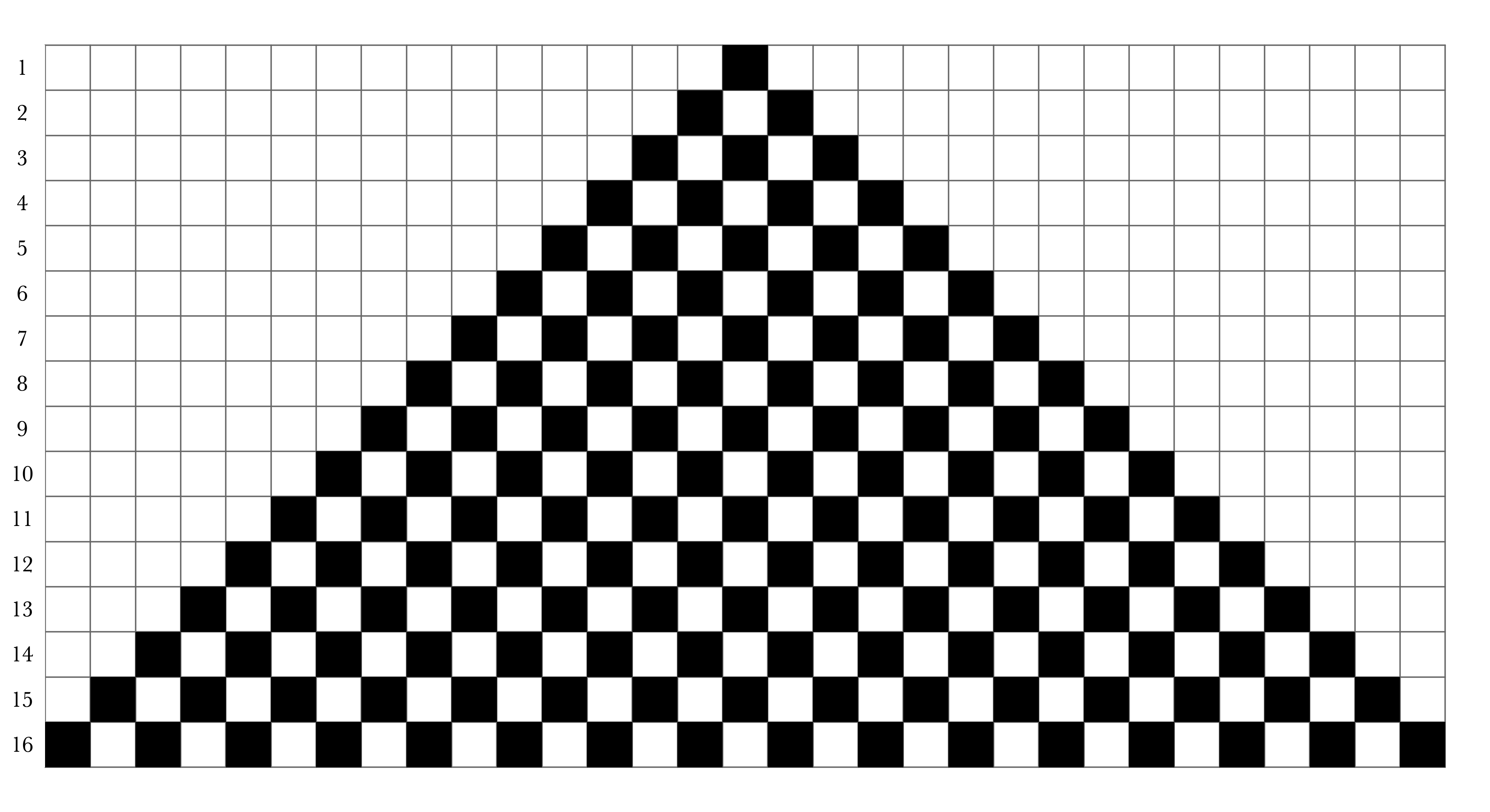
Given the specification of a rule as above and an initial configuration, we can simulate the execution of a cellular automaton by hand. Specifically, we can fill out a grid row-by-row where the state (color) of each cell in a row is determined according to the states of the three cells above it. For example, here are the first few steps of the rule depicted above, again with the initial configuration consisting of a single cell in state 1.

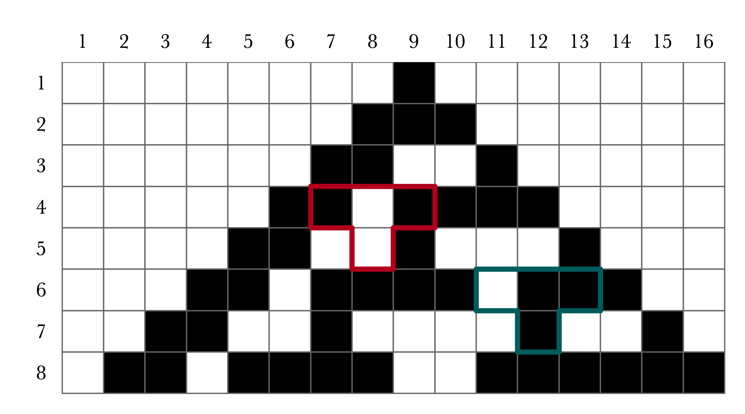
The two highlighted regions indicate how the values of cells relate to the rule depicted above. For example, the cell in step (row) 5 and cell (column) 8 is in state 1 because in the previous step, cell 8 was in state 0, while its neighbors were both in state 1. This corresponds to the figure labelled 5 in the rule above, which stipulates that cell 8 should set its state to 0 in step 5. Similarly, cell 12 in step 7 is in state 1 according to the figure labelled 3 in the depiction of the rule.

Naming of Cellular Automata

As shown above, a rule is specified by the values resulting from every possible configuration of the three consecutive cells. There are 8 such configurations, and for each configuration, there are 2 options for what the updated value should be (0 or 1). Thus, there are \(2^8 = 256\) possible (one-dimensional, two-state) cellular automata rules.

Following Wolfram, we number the possible rules Rule 0, Rule 1,…, Rule 255. The number associated to each rule is determined according to binary representation. For each of the possible configurations of three consecutive cells, write the resulting state for the middle cell:

1
2
3
4
5
6
7
8
  000: b0
  001: b1
  010: b2
  011: b3
  100: b4
  101: b5
  110: b6
  111: b7

Then interpret the resulting bits as a binary representation of an integer. That is, the rule number is

1
  rule = 128 * b7 + 64 * b6 + 32 * b5 + 16 * b4 + 8 * b3 + 4 * b2 + 2 * b1 + b0

For example, for this rule

We would have b4, b3, b2, b1 = 1 while the other values are 0. Thus this is Rule 30.

Exercise. Consider the rule defined as follows: if either of a cell’s neighbors are 1, then the cell updates its state to 1. Otherwise, the cell’s next state is 0. What is the number of this rule?

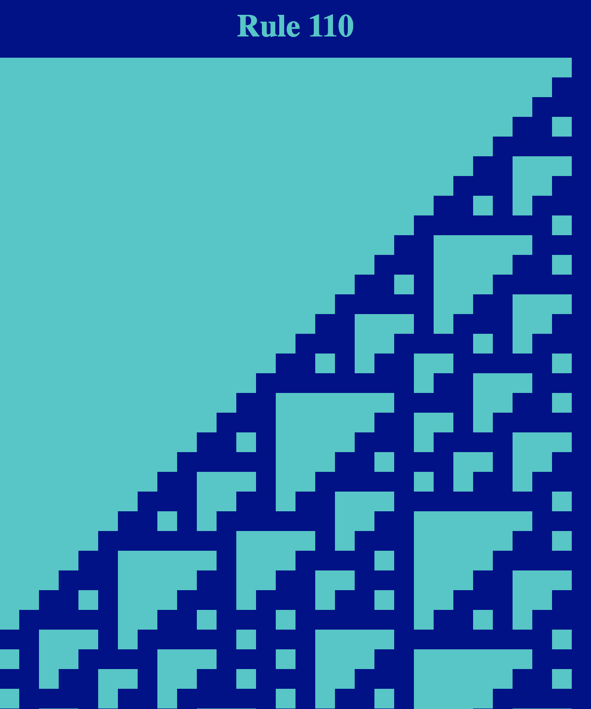
Exercise. Draw a diagram depicting Rule 110, and simulate a few steps of its execution with an initial configuration consisting of a single cell with state 1 and the remaining cells of state 0.

Applications and Surprises

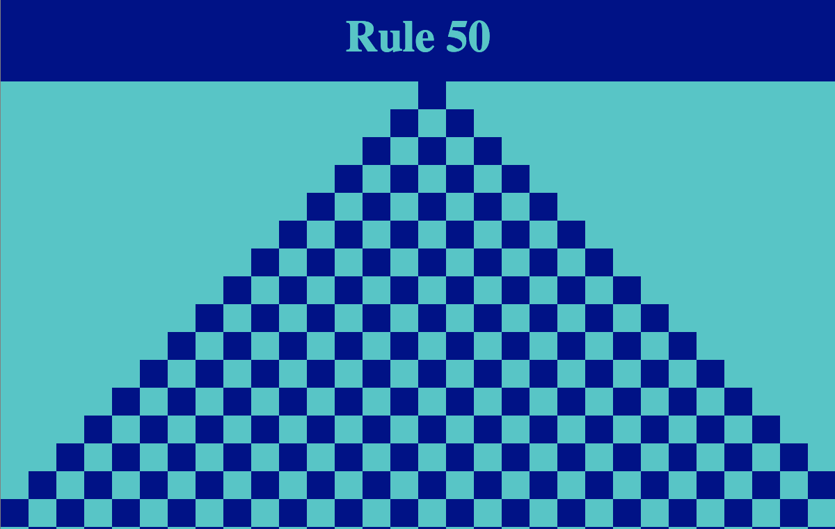
Cellular automata are defined by simple rules, so one might naturally expect that their behavior tends to be fairly predictable. Indeed, the space-time diagrams of may cellular automata simply produce very regular patterns (at least when the initial configuration is simple). For example, here is a very predictable pattern produced by Rule 50 when the initial configuration contains exactly one 1 value:

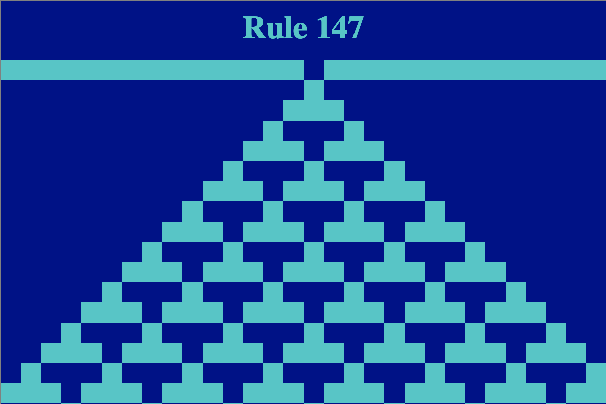
A slightly more interesting, but no less repetitive pattern is generated by Rule 147:

Even though these particular images may not be especially exciting or surprising, the rules for generating these patterns are so simple that they can be implemented incredibly efficiently by a computer program. Thus, if one finds a cellular automaton that makes a desired pattern, you might be hard pressed to find a simpler description of the pattern that simply specifying its associated rule number.

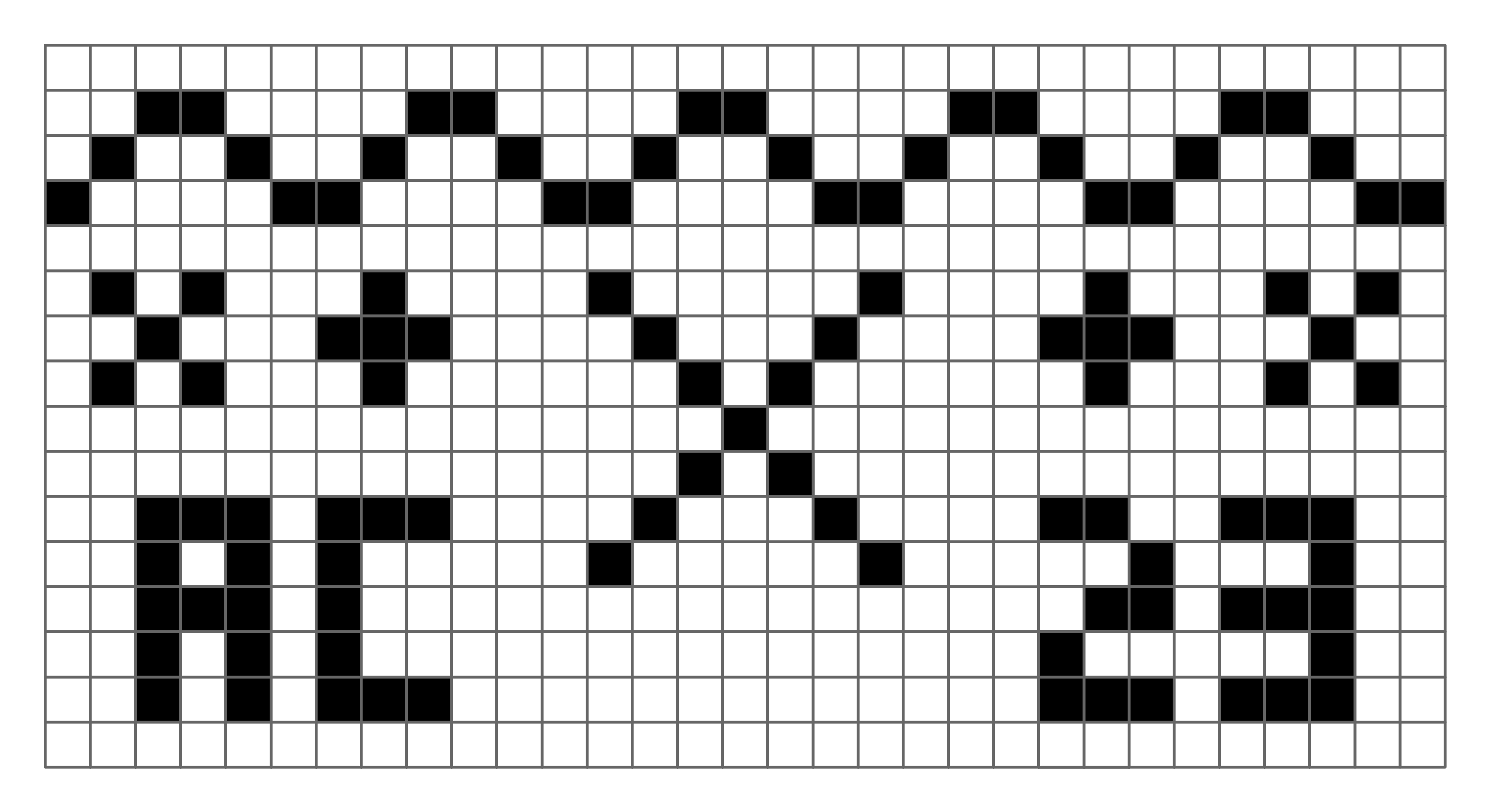
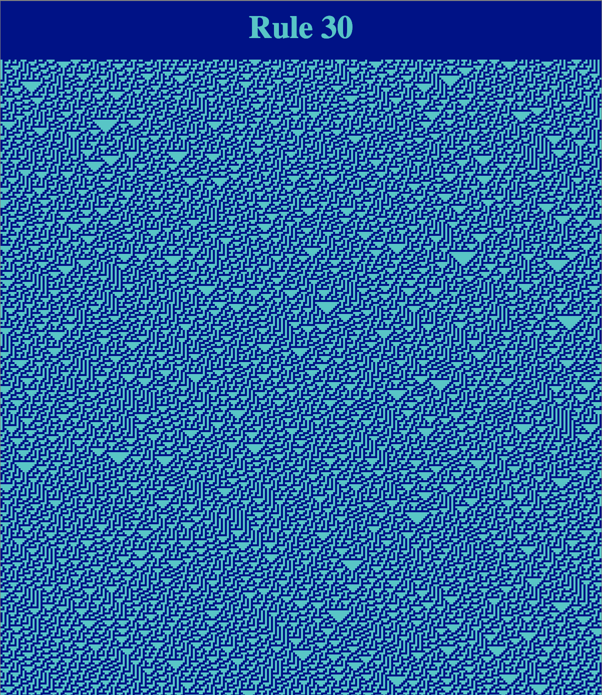
While the patterns depicted above are quite repetitive, a few rules demonstrate a surprising amount of complexity. For example, consider Rule 30:

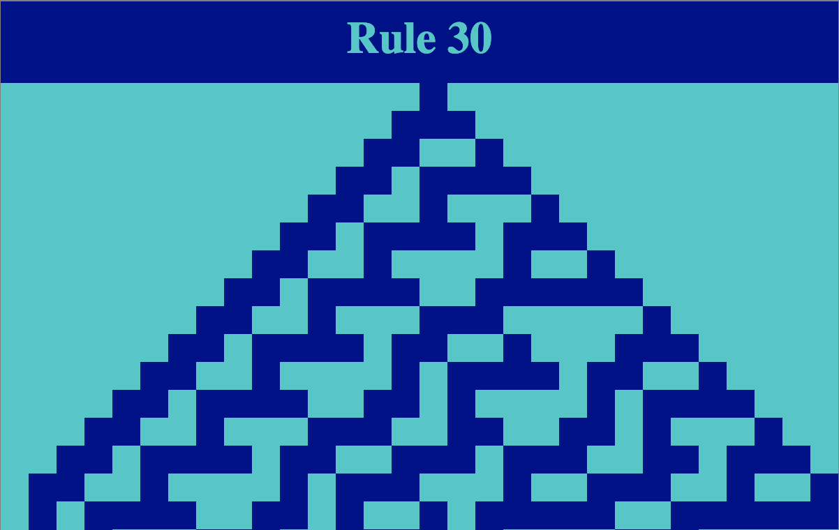
Even with a very simple initial condition (a single cell with value 1 and the rest 0), we begin to see some seemingly unpredictable behavior in the right half of the diagram. Running a larger system for more iterations, we see that the pattern appears to be more chaotic.

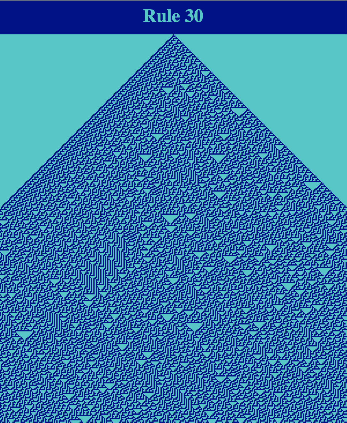
The visual appearance of this pattern is compelling as it has many patterns and textures that are repeated (e.g., downward facing triangles), but not in an obviously predictable manner. Despite the visual complexity of the figure, its description as a cellular automaton is simple. Further patterns and visual textures can be created by changing the initial configuration of the automaton. Here is an example execution of Rule 30 where the initial state of each cell is chosen randomly:

The image above shows how cellular automata can lend themselves well to generative design. In order to achieve a desired visual effect, one can choose a procedure (e.g., cellular automaton rule) and ``steer’’ the execution by choosing a suitable initial condition. Cellular automata have been employed in designing building facades, such as the Cambridge North train station in the UK (which used Rule 30.

Rule 30 has also been proposed as an explanation for the color patterns of certain seashells. Rule 30 was also studied as an efficient pseudo-random number generator, by Marco and Tomassini.

The illustrations above show that cellular automata can exhibit emergence: the idea that simple elements following simple rules can nonetheless display complex collective behavior. An extreme demonstration the emergent behavior of cellular automata is Rule 110:

Like Rule 30, Rule 110 seems to exhibit a balance between regular structure and chaotic behavior:

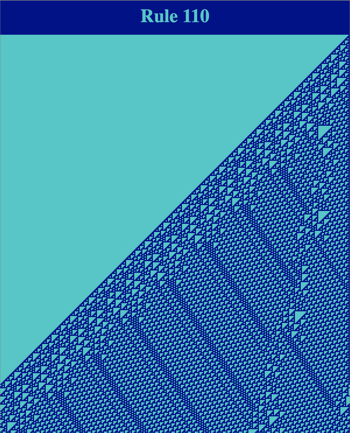
Rule 110, however, seems to have more predictable repeated patterns than Rule 30. In 2004, Matthew Cook proved that Rule 110 is a universal computer. In effect, what this means is that any computation that can be performed by any (deterministic) computer can be emulated by an appropriate execution of Rule 110. Cook’s analysis shows a network can be “programmed” by setting the initial configuration appropriately such that Rule 110 can perform any computation that can be performed by a (classical, deterministic) computer.