Midterm II Guide
Your guide to the second midterm
Overview
Midterm II will focus on the material covered since the first midterm. The main topics covered will be graph algorithms, greedy algorithms, and dynamic programming.
List of Topics
Greedy Algorithms
- Understand what a greedy algorithm is. and
- Devise a greedy procedure for solving a problem.
- Apply the “algorithm stays ahead” technique for arguing the correctness of a greedy algorithm.
- Understand and execute/simulate standard greedy algorithms by hand (see specific algorithms and problems below).
Relevant reading:
- AI Chapters 7, 9, 13, 15
- KT Chapter 4
- AA Chapter 4
Dynamic Programming
- Develop a recursive solution to an algorithmic problem.
- Memoize the recursive implementation and/or compute the solution iteratively by filling out a table.
- Argue the correctness and running time of your procedure.
- Execute a dynamic programming solution by hand to solve a concrete problem instance.
- Understand and execute/simulate standard dynamic programming algorithms by hand (see specific algorithms and problems below).
Relevant reading:
- AI Chapters 16, 17, 18
- KT Chapter 6
- AA Chapter 6
Specific Algorithms and Problems
Graph problems:
- Eulerian cycle
- shortest paths (directed/undirected, weighted/unweighted)
- minimum spanning trees
Optimization problems:
- profit maximization
- interval scheduling (weighted/unweighted)
- knapsack problem
- sequence alignment
Algorithms:
- breadth-first search
- Dijkstra’s algorithm
- Prim’s algorithm
- Kruskal’s algorithm
- greedy interval scheduling
- memoized profit maximization
- weighted interval scheduling via dynamic programming
- knapsack via dynamic programming
- sequence alignment via dynamic programming
- Bellman-Ford algorithm
Example Questions
Exercise 1. Consider the following graph \(G = (V, E)\).
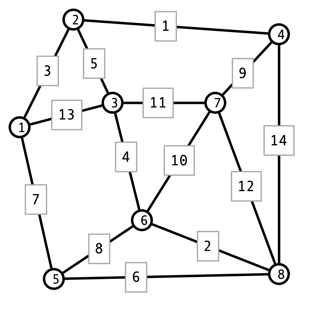
- Determine whether or not \(G\) contains an Eulerian circuit.
- Use Dijkstra’s algorithm to find the shortest path from vertex \(1\) to vertex \(8\).
- Use Prim’s algorithm to find a minimum spanning tree \(T\) starting from vertex \(1\). In what order does Prim’s algorithms add the edges to \(T\)?
- Use Kruskal’s algorithm to find a minimum spanning tree \(T\). In what order does Kruskal’s algorithm add the edges to \(T\)?
Exercise 2. Suppose \(a\) is an array of size \(n\). Let \(s\) be an array of size \(m \leq n\). We say that \(s\) is a subsequence of \(a\) if there are indices \(1 \leq i_1 < i_2 < \cdots < i_m \leq n\) such that \(s[1] = a[i_1], s[2] = a[i_2], \ldots, s[m] = a[i_m]\). For example, if \(a = [a, l, g, o, r, i, t, h, m, s]\), then \(s = [l, o, t, s]\) is a subsequence of \(a\), but \(s' = [l, o, s, t]\) is not. Devise an algorithm \(\mathrm{Subsequence}(a, s)\) that determines whether or not \(s\) is a subsequence of \(a\). The running time of your algorithm should be \(O(n)\) where \(n\) is the length of \(a\).
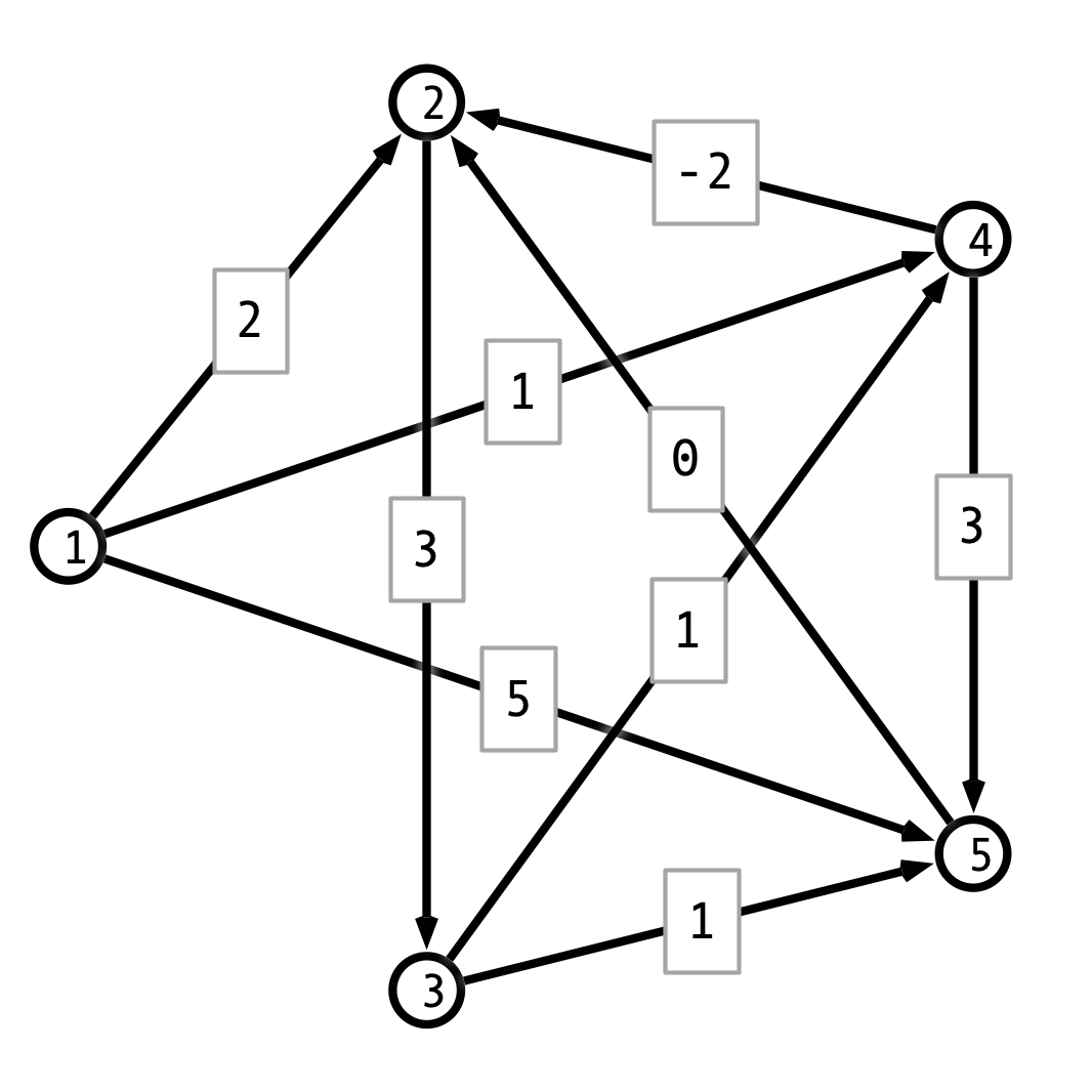
Exercise 3. Consider the following weighted, direccted graph.
-
Use Bellman-Ford to find a the shortest path from vertex \(1\) to vertex \(5\).
-
Modify the graph by adding \(2\) to each edge weight so that all edge weights are non-negative and find the shortest path from \(1\) to \(5\).
-
Explain why you find different shortest paths in the graphs from parts 1 and 2.
Exercise 4. Consider the following game. The board consists of a triangle of bricks, where each brick has an associated value. You begin at the uppermost brick, and you must choose a path from the top to the base of the triangle. Each step, you may only move downwards to one of the bricks immediately below your current location. Your goal is to choose a path that maximizes the sum of the values of the bricks along your path. The example below depicts an instance of the game with a triangle of height \(n = 7\). The highlighted path has a value of \(19\) (though I do not claim this to be the optimal path).
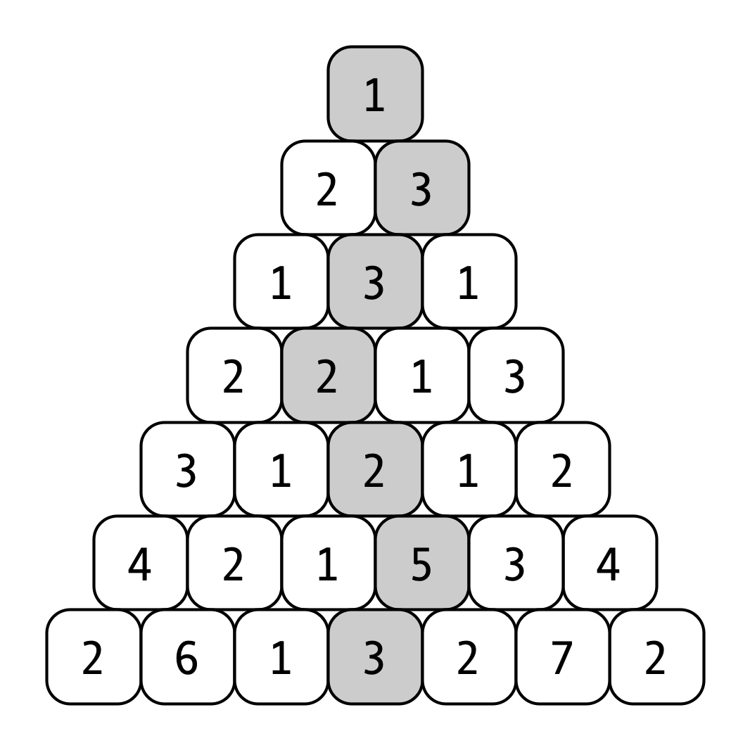
More formally, an instance of the game can be represented by a two-dimensional array \(a\) that stores the values of the bricks. For example \(a[n, 1]\) stores the value of the top brick, \(a[n-1, 1]\) and \(a[n-1, 2]\) store the values of the bricks on the next level down, etc. The example above woul have array representation as follows:
1
2
3
4
5
  a[7] = [1]
  a[6] = [2, 3]
  a[5] = [1, 3, 1]
       :
  a[1] = [2, 6, 1, 3, 2, 7, 2]
Observe that in general, given a brick with indices \((i, j)\) (i.e., the \(j\)th brick at height \(i\)), the two bricks immediately below it have indices \((i-1, j)\) and \((i-1, j+1)\). Thus, we can represented the highlighted path in the example as the sequence \((7, 1), (6, 2), (5, 2), (4, 2), (3, 3), (2, 4), (1, 4)\).
-
Devise a dynamic programming algorithm that finds the value of the optimal path from the triangle’s peak to base.
-
If the triangle has height \(n\), what is the running time of your procedure as a function of \(n\)?
-
Use your algorithm to determine the optimal path for the example depicted above.
Solutions
Solution 1.
-
\(G\) does not contain an Eulerian circuit. As we showed in class, a graph contains an Eulerian circuit if and only if all vertices have even degrees. Since vertex \(1\) has degree \(3\), the graph does not have an Eurlerian circuit.
-
Here is the output of Dijkstra’s algorithm:
The shortest path from \(1\) to \(8\) is the path \(1, 5, 8\), which has length 13.
-
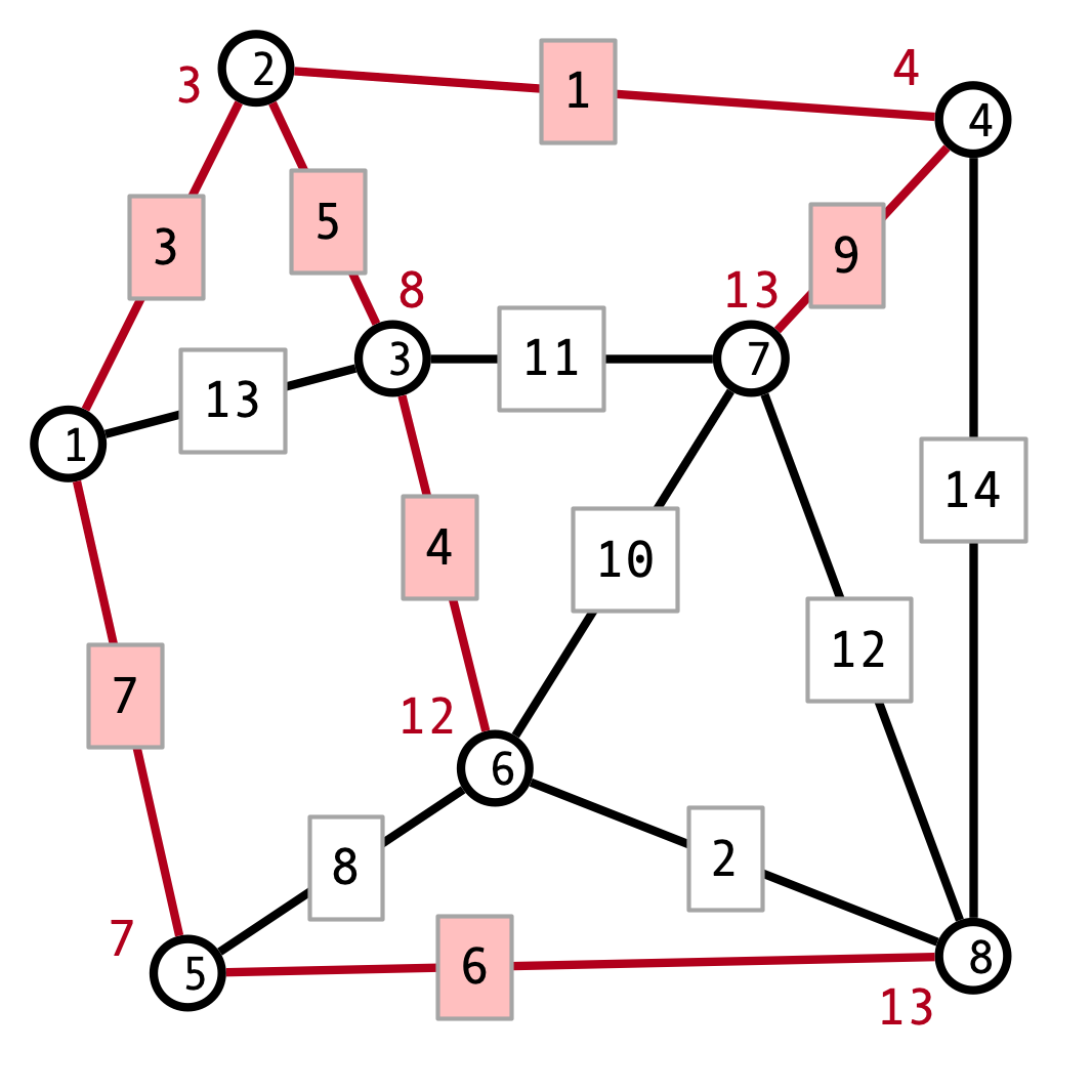
Here is a minimum spanning tree for the graph, produced by Prim’s algorithm:
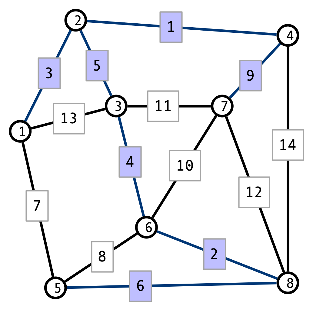
The edges were added in the following order: \((1, 2), (2, 4), (2, 3), (3, 6), (6, 8), (5, 8)\)
-
Kruskal’s algorithm produces the same output. However, in this case the edges were added in the order \((2, 4), (6, 8), (1, 2), (3, 6), (2, 3), (5, 8)\).
Solution 2. Consider the following greedy approach: match \(x = s[1]\) with the first appearance of \(x\) in \(a\) (if any). Then do the same with \(s[2]\), etc. If all entries in \(s\) are matched, then \(s\) is a substring of \(a\). Otherwise, if the end of \(a\) is reached without matching all characters of \(s\), then \(s\) is not a substring. We make this procedure more precise with pseudocode as follows:
1
2
3
4
5
6
7
8
9
10
11
  Subsequence(a, s):
    j <- 1
    for i from 1 to Size(a):
      if a[i] = s[j] then
        j <- j + 1
        if (j > Size(s)) then
          return true
        endfi
      endif
    endfor
    return false
To establish the correcntess of the procedure, first observe that if Subsequence(a, s) returns true, then then \(s\) is a subsequence of \(a\). To see this, observe that in order for the method to return true, we must have \(a[i_j] = s[j]\) for \(m\) values \(i_1 < i_2 < \cdots < i_m\).
On the other hand, suppose \(s\) is a subsequence of \(a\), with \(s[1] = a[i_1], s[2] = a[i_2], \ldots, s[m] = a[i_m]\). Then the condition \(a[i] = s[1]\) in line 4 is satisfied for some \(i \leq i_1\) (the first index at which \(a[i] = s[1]\)). Arguing by induction, we similarly find that for all \(k \leq m\), there is some index \(i \leq i_k\) for which the condition \(a[i] = s[k]\) holds in line 4. Thus Subsequence(a, s) returns true, as claimed.
Solution 3. Here is a table of the distnace values computed by Bellman-Ford on the original graph. The arrows indicate which incoming edge resulted in the minimal distance computation:
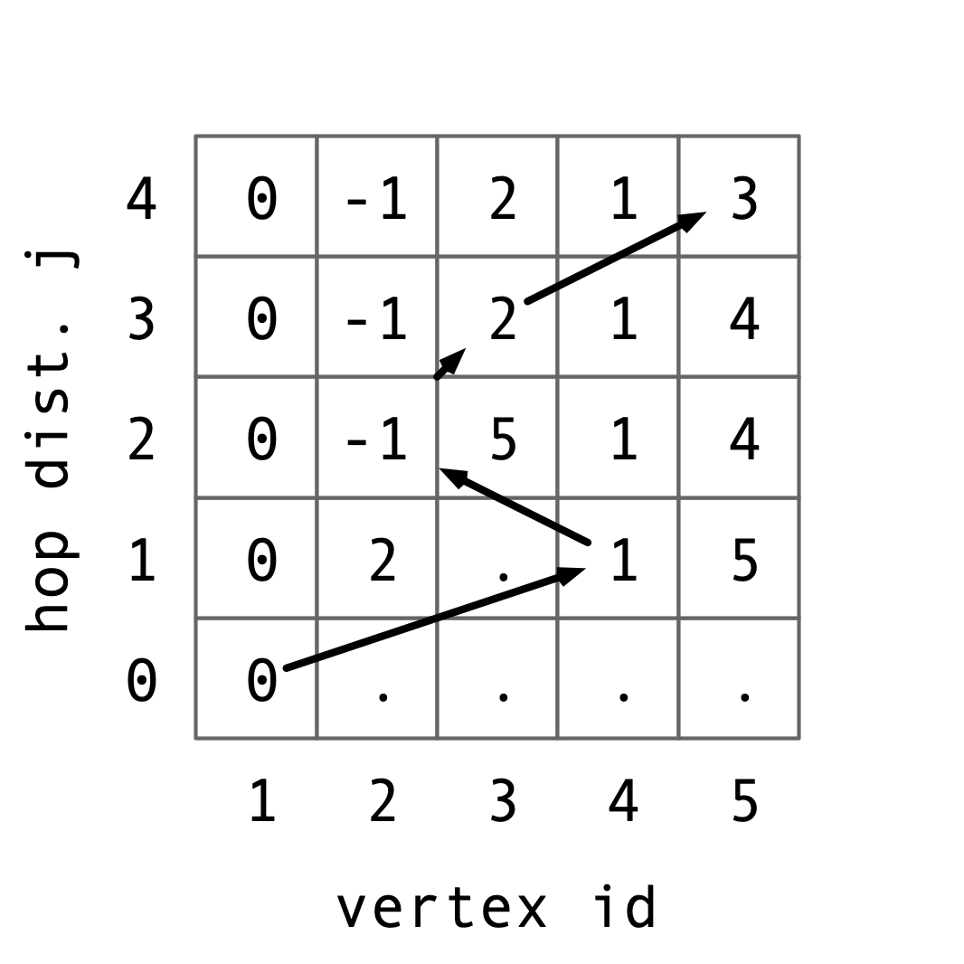
Thus, the shortest path from \(1\) to \(5\) is the path \(1, 4, 2, 3, 5\), which has (weighted) length 3.
Since the graph with edge weights increased by \(2\) has no negative weighted edges, we can use Dijkstra’s algorithm for shortest paths. We get the following output:
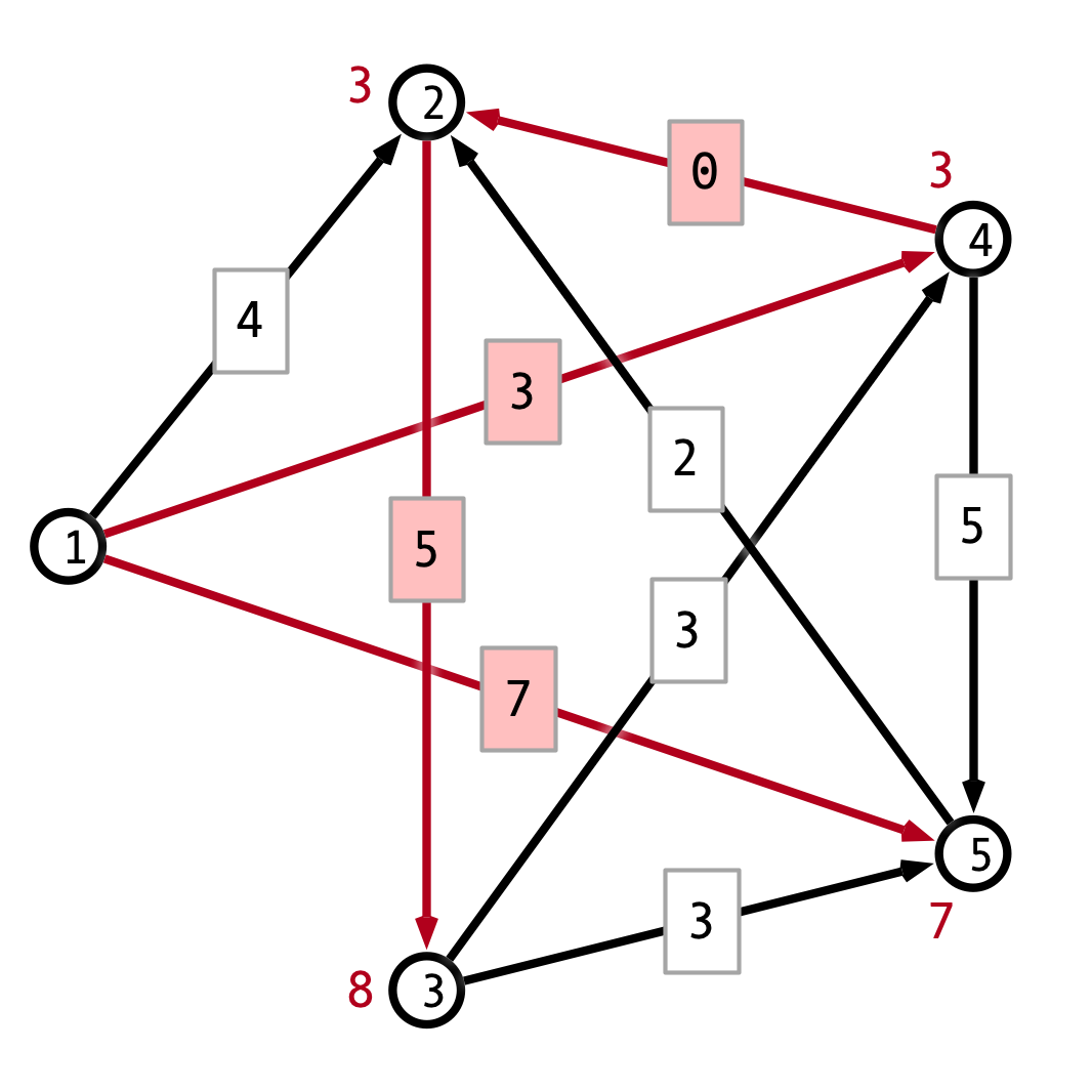
Thus, the shortest path is simply the edge from \(1\) to \(5\), which has length \(7\).
Adding the constant weight \(2\) to every edge in the graph changes the shortest paths because paths with more hops get more weight added to them. The original shortest path consisted of \(4\) hops, so its length increased by \(8 = 2 \times 4\) from \(3\) to \(11\). On the other hand, the one hop path length only increases by \(2\) from \(5\) to \(7\).
Solution 4. Towards developing an algorithm for the problem, first observe that starting from the top (with index \((n, 1)\)) the optimal solution will be the better of the optimal solutions when starting from \((n-1, 1)\) and \((n-1, 2)\) (the two bricks below the top), plus the value of the top brick \(a(n, 1)\). More generally, the optimal solution starting from any brick \((i, j)\) has value \(a(i, j)\) plus the maximum of the optimal solutions starting from the two bricks below, \((i-1, j)\) and \((i-1, j+1)\).
Let \(\opt(i, j)\) denote the optimal value achievable when starting from the brick with index \((i, j)\). Then \(\opt\) satisfies the following recursion relation
\[\opt(i, j) = a[i, j] + \max(\opt(i-1, j), \opt(i-1, j+1))\]where we interpret \(\opt(0, j) = 0\) for all \(j\).
We can compute the values of \(\opt(i, j)\) iteratavely using dynamic programming as follows. The two dimensional array b will store the values of \(\opt(i, j)\).
1
2
3
4
5
6
7
8
9
  MaxValue(a):
    n <- Size(a)
    b[1] <- a[1]
    for i = 2 up to n do:
      for j = 1 up to n - i + 1 do:
        b[i, j] = a[i, j] + Max(b[i-1, j], b[i-1, j+1])
      endfor
    endfor
    return b[n, 1]
The running time of this procedure is \(O(n^2)\), as there are \(n - 1\) iterations of the outer loop, and at most \(n - 1\) of the inner loop in each outer loop iteration.
Applying this procedure to the example given results in the following table of values of b:
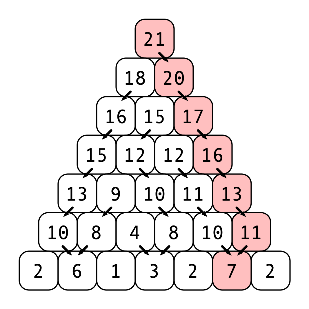
The arrow at each entry b[i, j] indicates which value (b[i-1, j] or b[i-1, j-1]) achieved the maximum in line 6. The path achieving the maximum total value is highlighted.