Homework 01

Download this assignment in pdf format or .tex source.

Exercise 1. Recall that a complete binary tree of height \(h\) is a tree in which all internal nodes have two children, and every leaf is at distance \(h\) from the root. For example, here are complete binary trees of height 0, 1, 2, and 4.

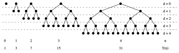
For \(n = 0, 1, 2, \ldots\), let \(T(n)\) denote the number of nodes in a complete binary tree of height \(n\). For example, we have \(T(0) = 1, T(1) = 3, T(2) = 7, T(3) = 15\). Observe that at each depth \(d\), a complete binary tree has \(2^d\) nodes at depth \(d\). Thus, we can express

Find a (simple!) general expression for \(T(n)\) and prove that your expression is correct using induction.

Exercise 2. Consider the following functions:

1. Sort the functions above by asymptotic growth. That is, write the functions in order \(f_{i_1}, f_{i_2}, \ldots\) such that \(f_{i_1} = O(f_{i_2})\), \(f_{i_2} = O(f_{i_3})\), etc.

2. Consider the function

   \[g(n) = \begin{cases} n &\text{ if } n \text{ is odd}\\ \sqrt{n} &\text{ if } n \text{ is even} \end{cases}\]

   Which functions \(f_i\) satisfy \(f_i = O(g)\)? Which functions satisfy \(g = O(f_i)\).

3. Find a function \(h(n)\) such that neither \(h = O(g)\), nor \(g = O(h)\).

Exercise 3. In this exercise you will explore the empirical running times of four sorting algorithms:

1. insertion sort
2. selection sort
3. bubble sort
4. merge sort

To answer the following questions, you may write your own implementation of these sorting procedures or use a provided implementation in Java (Sorting.java and SortTester.java). (It is easy enough to find implementations of these procedures in most popular languages on the web as well.) You do not have to submit your code for this exercise.

1. Write a program that records the running times of the four sorting algorithms for a two ranges of arrays sizes:

   • arrays of size up to 100 (small inputs)
   • arrays of size up to 100,000 (large inputs)

   Use the output of your program to graph and compare the emprical running times of the four algorithms over the ranges of sizes. For various sizes in the range (say 5, 10, 15,…,100 for small input, 5,000, 10,000,…,100,000 for large), generate arrays of random integers and record how long each algorithm takes to sort the array. Generate two plots: one that shows the running times for small inputs, and one for large. For the purposes of comparing running times, you should include the data for all four algorithms on the same plot. For small inputs, you may see a lot of variability in the running times. To get a more accurate picture of the trend, I suggest doing many trials at each size (my example does 1000), and record the average running times. Be sure you use a new random array for each trial!

2. The worst-case asymptotic running times of insertion, selection, and bubble sort are \(O(n^2)\), while merge sort runs in \(O(n \log n)\). Are your graphs for large inputs consistent with these trends? What about for the small inputs? Which algorithm is fastest for smaller inputs?

3. Comparing only insertion, selection, and bubble sort, which tends to be fastest for small inputs? For large inputs? How can you explain this trend? Refer to the (pseudo)code of the procedures to justify your response. (Keep in mind that your trends are for randomly generated arrays.)

4. Examining the (pseudo)code for insertion, selection, and bubble sort, can you describe a (very large) input that you would expect one of these three algorithms to be significantly faster than the others? Might this algorithm even be faster than merge sort on your input?

5. Assuming you found a sorting procedure that is more efficient than merge sort on small inputs, how could you use this procedure to modify merge sort to be more efficient on large inputs?

Exercise 4. In the sorting algorithms we’ve considered so far, we have assumed that values are stored in an array \(a\) that support the operation \(\swap(a, i, j)\) for all possible indices \(i\) and \(j\). However, some data structures—e.g., linked lists—may only support adjacent swaps i.e., swaps for the form \(\swap(a, i, i+1)\). We can still sort an array using adjacent swaps; for example InsertionSort only ever uses adjacent swaps. For every \(n\), describe an array of length \(n\) such that every sorting algorithm that modifies the array using only adjacent swaps requires \(\Omega(n^2)\) adjacent swaps to sort in the worst case.

Hint. We say that indices \(i, j\) form an inversion if \(i < j\) and \(a[i] > a[j]\). For example, the array \(a = [6, 8, 5, 7]\) has 3 inversions: \((1, 3)\), \((2, 3)\), \((2, 4)\). If \(a\) has \(k\) inversions, how many fewer inversions could \(a\) have after performing a single adjacent swap? How many inversions can an array of length \(n\) have?