Lab 02: Computing Shortcuts

DUE: Friday, March 12, 23:59 AoE

Background

Suppose we have a network consisting of \(n\) nodes and directed links or edges between each pair of nodes. That is, given nodes \(i\) and \(j\), there is an edge \(e = (i, j)\) from \(i\) to \(j\). For example, the following figure illustrates a network with three nodes, and the arrows indicate the directions of the links: \((i, j)\) is indicated by an arrow from \(i\) to \(j\), while \((j, i)\) is indicated by an arrow from \(j\) to \(i\).

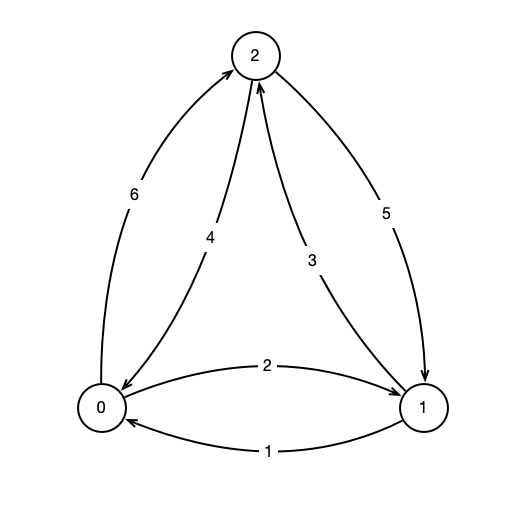
Each edge \((i, j)\) has an associated weight, \(w(i, j)\) that indicates the cost of moving from node \(i\) to node \(j\) along \((i, j)\). The weights of the edges are indicated in the figure above. For example, \(w(0, 1) = 2\). Given the weights of the edges, it might be the case in order to move from \(i\) to \(j\), it would be less expensive to travel via an intermediate node \(k\), i.e. travel from \(i\) to some \(k\), then from \(k\) to \(j\). Traveling in this way, we incur a cost of \(w(i, k) + w(k, j)\). For example, in the figure above, traveling from \(0\) to \(2\) across the edge \((0, 2)\), we incur a cost of \(w(0, 2) = 6\), while traveling from \(0\) to \(1\) to \(2\) has a cost of \(w(0, 1) + w(1, 2) = 2 + 3 = 5\). Thus, the path \(0, 1, 2\) is a shortcut from \(0\) to \(2\).

In this assignment, you will write a program that, given any network and weights, computes the cheapest route between every pair of nodes along a path of length at most 2 (i.e., with at most a single intermediate node).

Network Representation

We assume that the edge weights are positive real numbers (i.e., decimals). For a network with \(n\) nodes labeled, say \(1, 2, \ldots, n\), we must specify the weights \(w(i, j)\) for all \(i, j \leq n\). By convention, we take \(w(i, i) = 0\) for all \(i\). We can represent the network as an \(n \times n\) matrix \(D\)—i.e., a 2 dimensional \(n\) by \(n\) array of numbers. The entry in the \(i\)th row and \(j\)th column, \(d_{ij}\) stores the weight \(w(i, j)\). For example, here is the matrix corresponding to the previous figure:

If \(D\) represents the original matrix of weights, then the shortcut distances can also be represented by a matrix \(R\), where the entry \(r_{ij}\) stores the shortcut distance from node \(i\) to \(j\). More formally,

Notice that by taking \(k = i\), we have \(r_{ij} \leq d_{ii} + d_{ik} = d_{ik}\), because we assume \(d_{ii} = 0\). Using the \(D\) from our previous example, we compute the corresponding \(R\):

Notice that \(D\) and \(R\) are the same, except that \(d_{0, 2} = 6\), while \(r_{0, 2} = 5\). This corresponds to the shortcut \(0 \to 1 \to 2\) which has weight \(5\).

Internally, we can represent the original matrix as a two dimensional array of floats, e.g., with float[][] matrix = new float[n][n];. For the previous examples, we’d store \(D\) as follows.

1
2
3
[[0.0, 2.0, 6.0],
 [1.0, 0.0, 3.0],
 [4.0, 5.0, 0.0]]

A Note on Efficiency

Given an \(n \times n\) matrix \(D\), the resulting shortcut matrix \(R\) can be computed by taking the minimum \(r_{i j} = \min_{k} d_{i k} + d_{k j}\) directly. For each pair \(i, j \leq n\), taking this minimum requires \(n\) additions and comparisons: one addition and comparison for each value of \(k\). Thus the total number of elementary operations (floating point arithmetic, comparisons, etc.) is \(O(n^3)\). Therefore, even for a fairly modest network size of \(n \approx 1,000\), we already need billions of elementary operations. For a network of size 10,000, we need to perform trillions of operations. For reference, the network of city streets in New York City contains approximately 12,500 intersections with traffic signals (i.e., nodes), so naively computing shortcuts for New York would already require trillions of operations. (The structure of New York City streets allows for more efficient means of computing shortcuts, but this example shows the scale of a real-world application to finding shorter routes, say, for driving directions.)

Program Description

For this assignment, you will write a program that, given a matrix \(D\) (i.e., 2d array) of non-negative weights of edges, computes the shortcut matrix \(R\) as described above. Specifically, you will complete an implementation of the SquareMatrix class provided below by writing a method getShortcutMatrixOptimized (), that returns a SquareMatrix instance representing the shortcut matrix of this instance. To get started, download the SquareMatrix.java:

• SquareMatrix.java

Notice that there are actually two missing methods! We will code getShortcutMatrixBaseline() together in class.

• See baseline implementation below

Testing Your Program

Once you/we have implemented getShortcutMatrixBaseline() and getShortcutMatrixOptimized(), you can test your code using the following ShortcutTester program:

• ShortcutTester.java

This program will allow you to test the correctness and performance of getShortcutMatrixOptimized () compared to getShortcutMatrixBaseline(). Specifically, the program runs both shortcut computing methods several times on several input sizes and reports (1) the average run-time of the optimized method, (2) the run-time improvement fa compared to baseline, (3) the number of iterations performed per microsecond (where an iteration consists of single \(\min\) computation in the definition of \(r_{ij}\) above), and (4) whether or not the optimized method produces the same output as the baseline (it should!).

Hints and Resources

There are two main ways to improve the performance of getShortcutMatrixOptimized () compared to the baseline implementation. The first is to use multithreading. As we saw in Lab 01: Estimating Pi, multithreading can give a sizable speedup for performing operations that can be done parallel. Your optimized method should employ multithreading. Specifically, think about how to break up the task of computing \(D\) into sub-tasks that can be performed in parallel.

We also saw that depending on your own computer hardware, using different numbers of threads will give the best performance. Specifically, your computer cannot perform more threads in parallel than it has (virtual) cores. Since the number of cores varies from computer to computer, it is helpful to know how many processors are available to your program. Thankfully, Java can tell you using the Runtime class. Specifically, the Runtime class provides a method, availableProcessors() which will return the number of processors available on the machine running the program. Using a number of threads roughly equal to this number will tend to give the best performance (assuming you aren’t concurrently running other computationally intensive tasks). You can get the number of available processors by invoking

1
Runtime.getRuntime().availableProcessors();

For relatively small instances (\(n\) up to around 1,000 on my computer), multithreading alone leads to a pretty good performance boost. However, the performance is worse on larger instances. In one run, the baseline program took 2.2s on an instance of size 1024, while an instance of size 2048 took 54.7s. Given the basic algorithm we are applying, we would expect that doubling in instance size increases the number of operations performed by a factor of about \(8 (= 2^3)\). However in this case, doubling the instance size led to a factor 25 increase in run-time. The main reason for this unwelcome slow-down comes down to exactly how modern computers access items stored in their memory through a process of caching. In class (and in a forthcoming note) will discuss caching and how we can improve the performance of our program by making the program behave in a way consistent with how our system expects our program to behave.

What to Turn In

Be sure to turn in:

1. SquareMatrix.java with getShortcutMatrixOptimized() implemented and commented.
2. Other .java files defining other classes (you will probably have one implementing the Runnable interface).
3. A README file (plain text or markdown format) that describes the optimizations you made, and the effect you saw that these optimizations had. Please also mention changes, experiments, or tests you made even if they negatively affected your programs performance. This file need not be more than a couple short paragraphs of texts, but it should document the main parts of your program’s development.

Grading

Your programs will be graded on a 7 point scale according to the following criteria:

• Correctness (2 pts). Your program compiles and completes the task as specified in the program description above.

• Style (1 pt). Code is reasonably well-organized and readable (to a human). Variables, methods, and classes have sensible, descriptive names. Code is well-commented.

• Performance (2 pts). Code performance is comparable to the instructor’s implementation. Program shows a significant improvement in performance with multiple threads.

• Documentation (2 pts). Submission includes a README file indicating (1) the main optimizations made over the baseline implementation, (2) the effect of these optimizations (individually and together), and (3) any other optimizations tested, whether or not they had a positive, negative, or insignificant effect on the program performance. The document should be concise (not more than a couple short paragraphs are necessary), but it should give an indication of the optimizations you tested, what worked, and what didn’t.

Extension (Extra Credit)

The program above suggests finding shortcuts consisting of 2 “hops” in a network. However, we might wish to find shortcuts that include 4 hops. For example, maybe we have \(w(1,2) = 6\), while \(w(1,3) = w(3, 4) = w(4, 2) = 1\), so it would be less costly to travel from 1 to 2 along the path \(1 \to 3 \to 4 \to 2\). More generally, we might wish to find the cost of the cheapest path from every node \(i\) to every other node \(j\), no matter how many hops the path contains. This is problem is referred to as the all pairs shortest paths problem.

Using your getShortcutMatrixOptimized() method as a sub-routine, write a method that computes the weight of the cheapest path between every pair of nodes in the network. Your method should return a SquareMatrix whose \(ij\)-entry is the total weight of the cheapest path from node \(i\) to node \(j\).

Hint. Suppose d is the original SquareMatrix, and

1
r = d.getShortcutMatrixOptimized()

What does r.getShortcutMatrixOptimized() compute? Also, what is the longest length (i.e., maximum number of hops) that a cheapest path from \(i\) to \(j\) could be?

Baseline Implementation

1
2
3
4
5
6
7
8
9
10
11
12
13
14
15
16
17
18
19
20
21
22
23
24
25
26
27
    public SquareMatrix getShortcutMatrixBaseline () {

	int size = matrix.length;
	
	float[][] shortcuts = new float[size][size];

	for (int i = 0; i < size; ++i) {
	    for (int j = 0; j < size; ++j) {

		float min = Float.MAX_VALUE;
		
		for (int k = 0; k < size; ++k) {
		    float x = matrix[i][k];
		    float y = matrix[k][j];
		    float z = x + y;

		    if (z < min) {
			min = z;
		    }
		}

		shortcuts[i][j] = min;
	    }
	}
	
	return new SquareMatrix(shortcuts);
    }