Lecture 32: Bipartite Matchings and Reductions
COSC 311 Algorithms, Fall 2022
Overview
- Reductions
- Maximum Bipartite Matchings
- Reduction to Maximum Flow
Big Picture, So Far
Efficient algorithms for many problems:
- sorting
- graph problems
- shortest paths
- Eulerian circuits
- minimum spanning trees
- interval scheduling
- sequence alignment
- stable matching
All solved in $O(N^2)$ time ($N = $ size of instance)
A Question
What algorithmic problems cannot be solved efficiently?
-
What do we mean by “efficiently?”
-
How could we show that no algorithm can solve a problem efficiently?
- What is an “algorithm,” anyway?
Last Unit of the Semester
Algorithmic Reality
For many practical problems:
- no efficient algorithm is known
- no proof that there isn’t an efficient algorithm
What do we do in this situation?
Reductions & NP Completeness
- focus on relationships between problems
- what does it mean for problem $A$ to be no harder/easier than problem $B$?
Algorithm Life
Observation. Algorithm design is challenging.
Lifestyle Choice. Avoid designing new algorithms (when you can get away with it).
How?
Idea. Given a new problem $A$, transform it into a problem $B$ you already know how to solve!
Example from homework: Scheduling contractors with bids
Reductions
Properties of nice transformations:
- transforming instances of $A$ to instances of $B$ can be done efficiently
- solution to $B$ instance can be efficiently transformed back to solution for $A$ instance
$1 + 2 = $ reduction from problem $A$ to problem $B$
Coarse notion of efficiency:
- transformations can be done in time $O(N^c)$ for some constant $c$ ($N = $ input size)
In this case reduction is polynomial time reduction
- write $A \leq_P B$ if polynomial time reduction from $A$ to $B$
Practical Value of Reductions
If $A \leq_P B$, then:
- any efficient solution to $B$ gives an efficient solution to $A$
- an improved algorithm for $B$ may give an improved algorithm for $A$
New Challenge
- Given a problem $A$, solve it by reducing to another problem $B$ that you already have an algorithm for
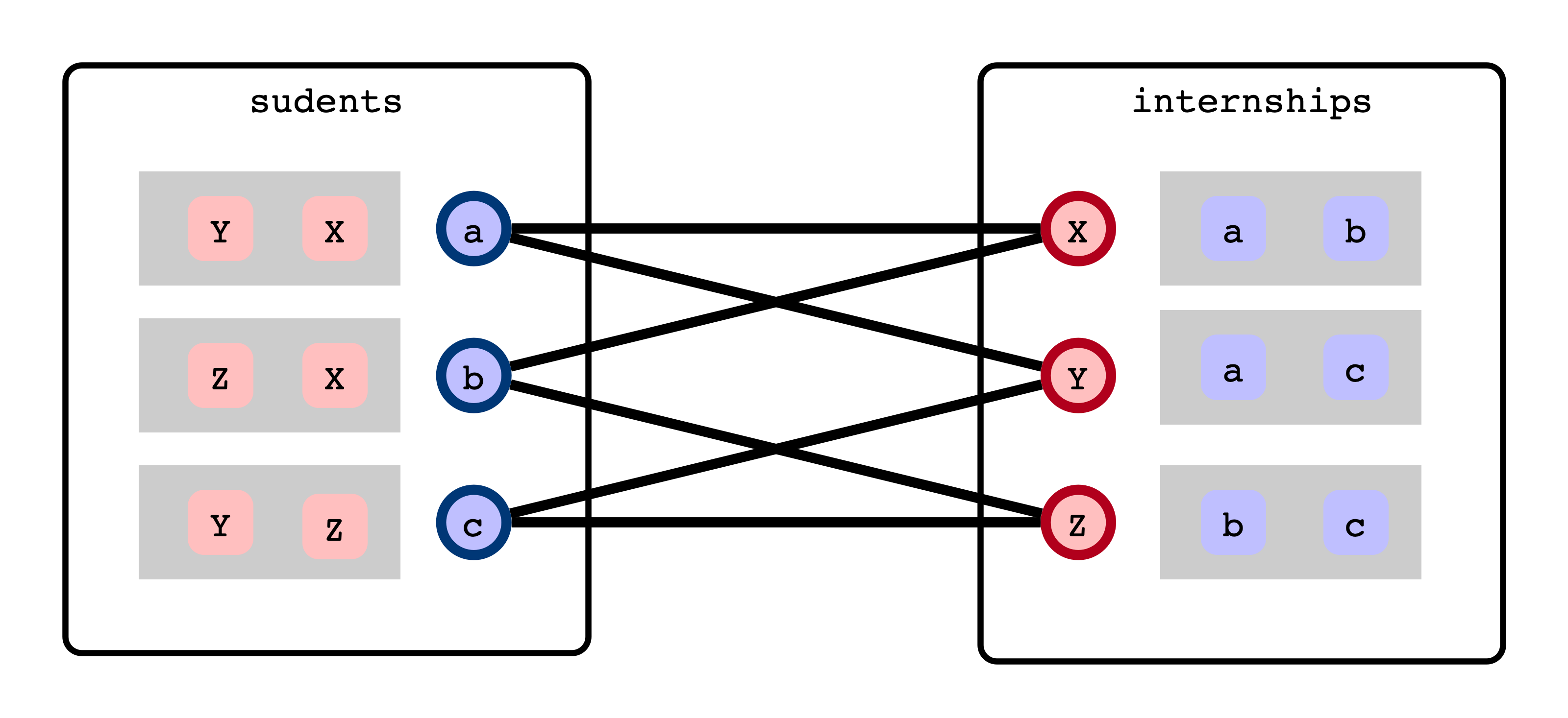
Internship Assignments, Again
In a small world…
- Three students: $a, b, c$
- Three internships: $X, Y, Z$
Students/Internships have acceptability criteria (not preferences)
- $a: Y, X$
- $b: Z, X$
- $c: Y, Z$
- $X: a, b$
- $Y: a, c$
- $Z: b, c$
How to match students an internships?
Viewed as a Graph
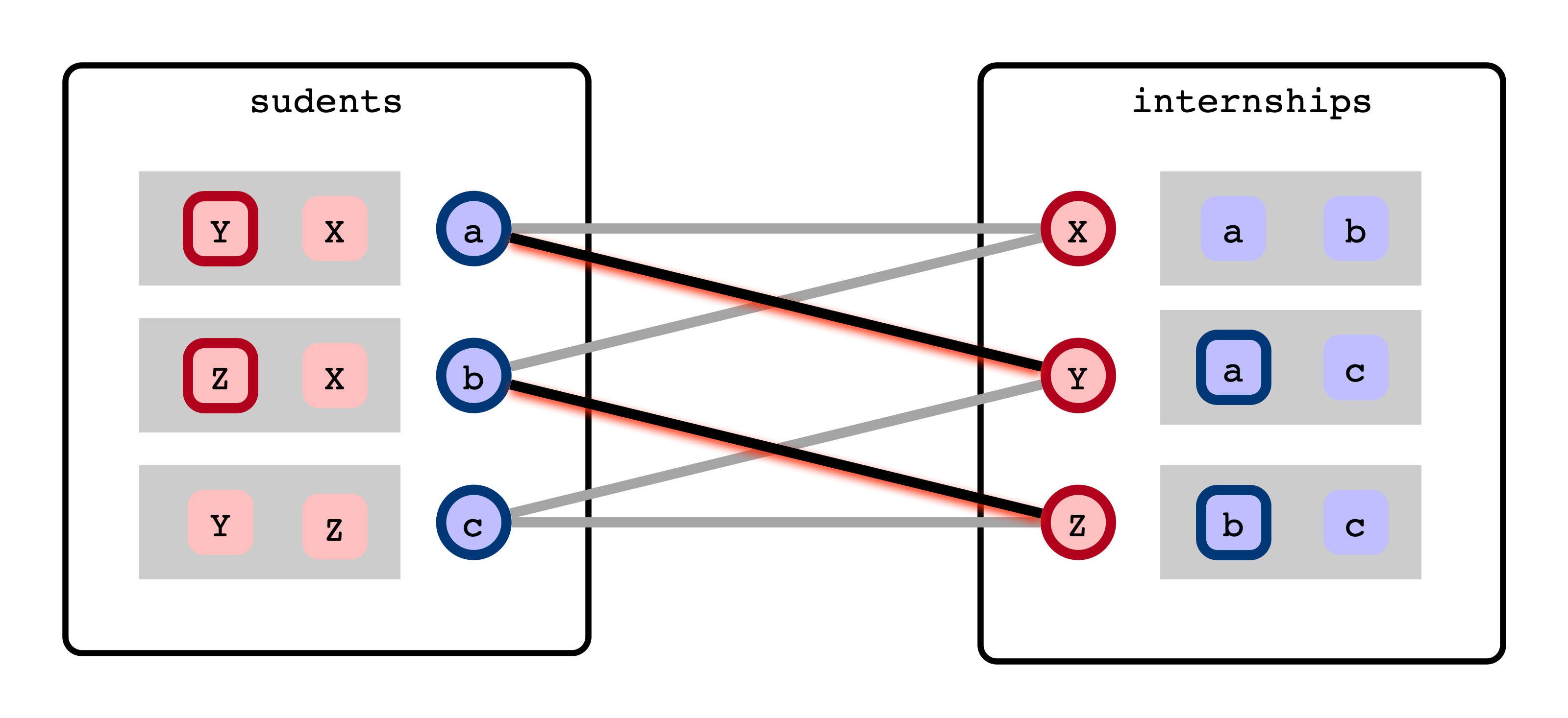
Not Great Matching
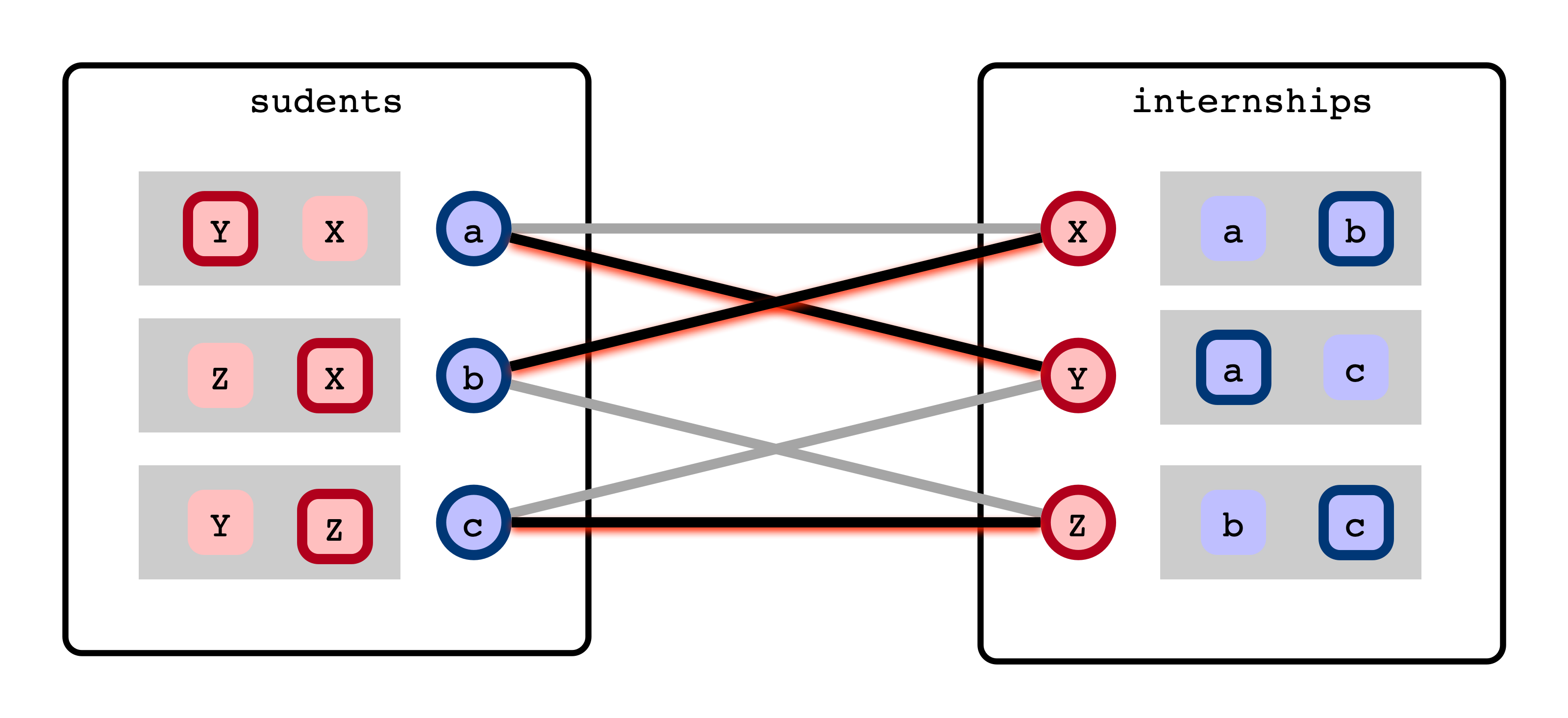
Best Matching
Maximum Bipartite Matching (MBM)
Input:
- bipartite graph $G = (V, E)$
- $V$ partitioned into two disjoint sets, $S, T$
- All edges are pairs $(s, t)$ with $s \in S$, $t \in T$
Output:
- a matching $M = \{(s_1, t_1), (s_2, t_2), \ldots, (s_k, t_k)\}$
- each $(s_i, t_i)$ is an edge in $G$
- each $s \in S$, $t \in T$ appears in at most one pair
- $M$ is a maximum matching: there is no matching of size $\ell > k$
Simplest Interesting Example
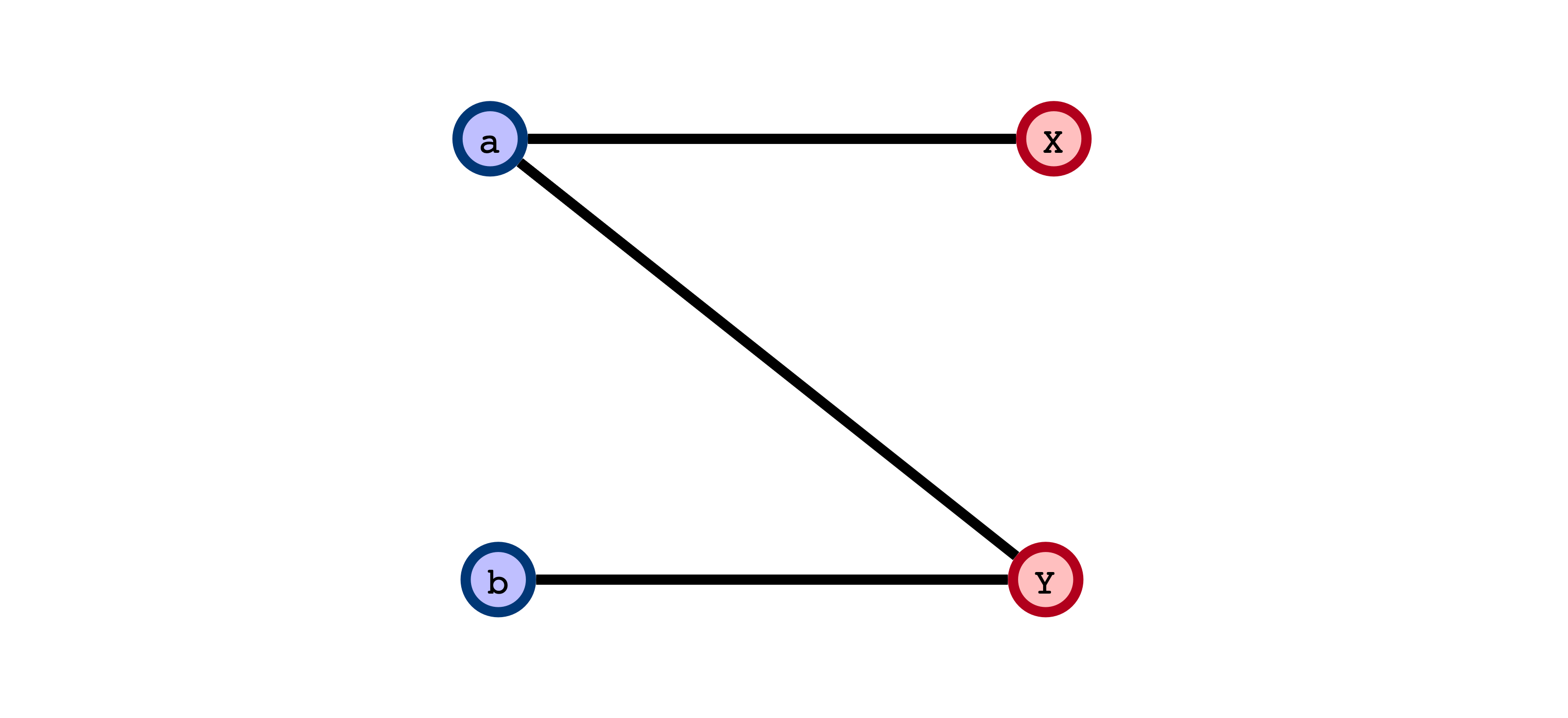
Does greedily adding edges to form a matching always result in a maximum matching?
Greedy Doesn’t Work
Issue: choosing an edge greedily/prematurely may block other edges that could result in a larger matching
- does this sound familiar?
Adapting to Our New Lifestyle
Don’t design a new algorithm…
…instead make a reduction to…
Maximum Flow!
Reduction to Max-Flow
How to turn MBM into a flow problem?
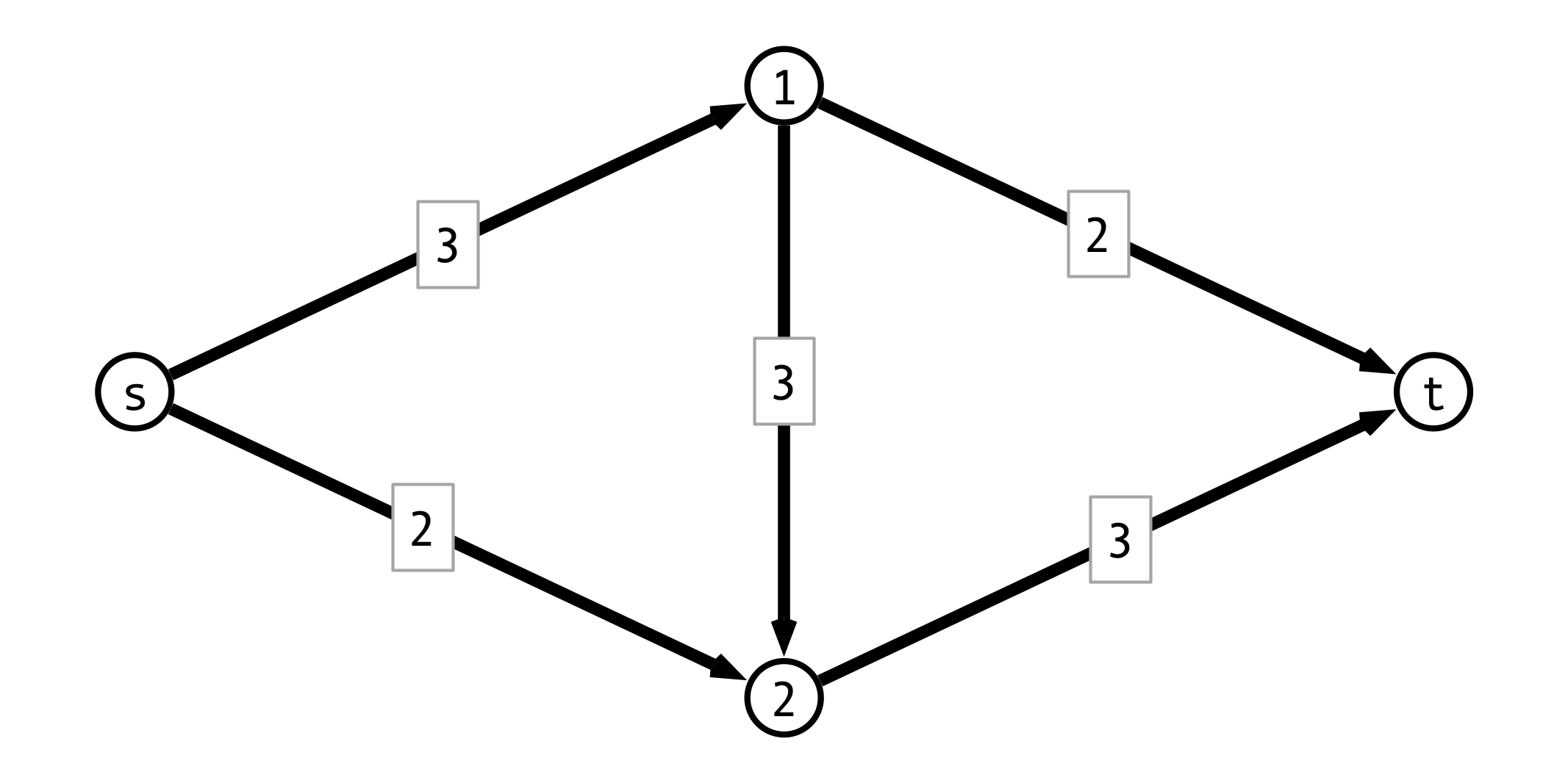
A Max-Flow Instance
Formalizing the Reduction
Input:
- Bipartite graph $G = (V, E)$ with $V = S \cup T$
Output:
- Directed graph $G’ = (V’, E’)$
- $V’ = V \cup \{s, t\}$
- For $E’$:
- direct all edges $(s_i, t_j) \in E$ from $S$ to $T$
- add edges $(s, s_i)$ for all $s_i \in S$
- add edges $(t_j, t)$ for all $t_j \in T$
- all capacities are $1$
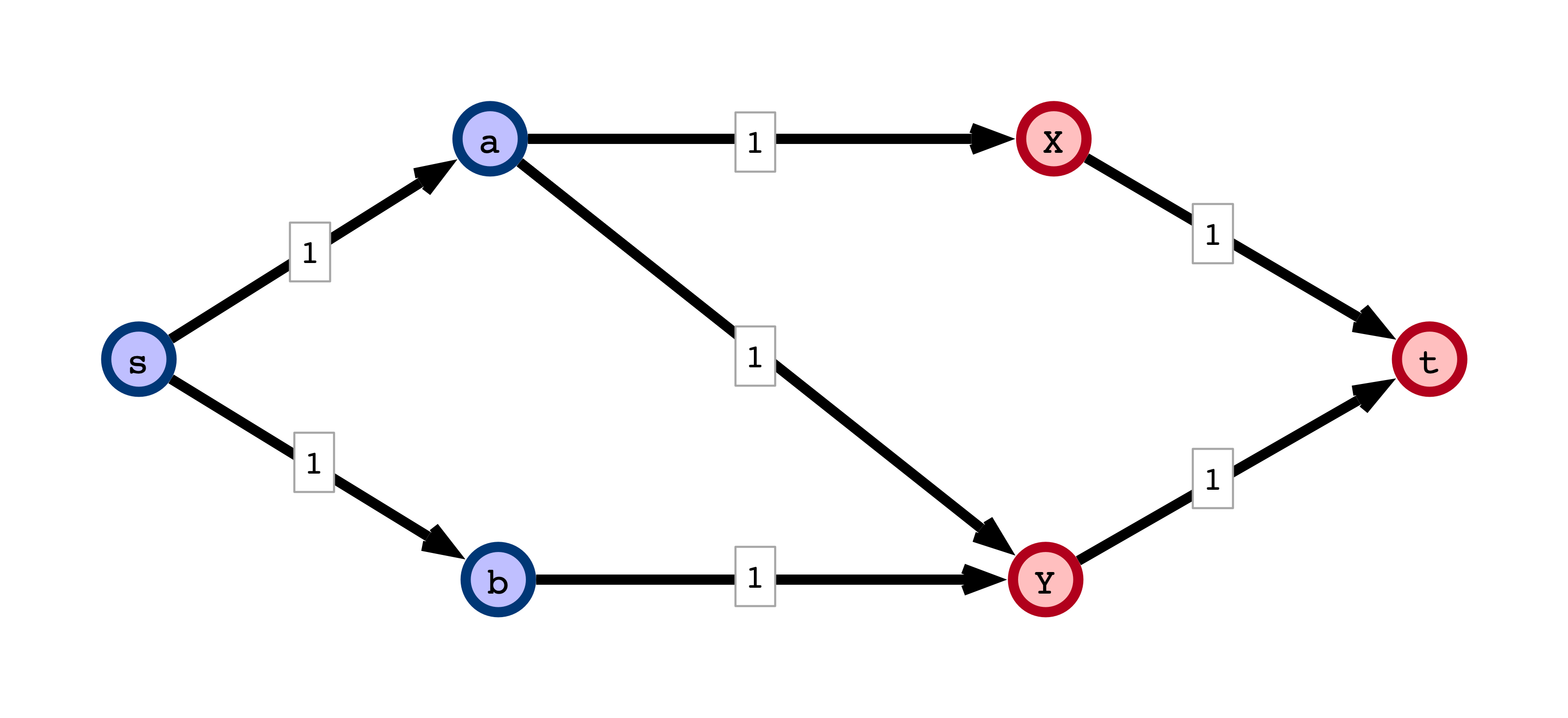
I Start with Bipartite Graph
II Form Max Flow Instance
III Solve Max Flow
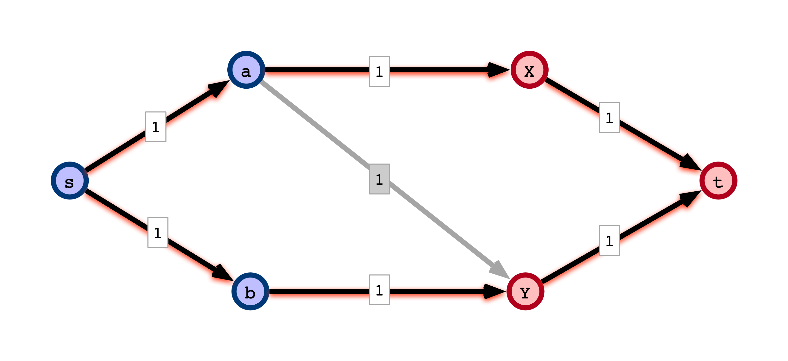
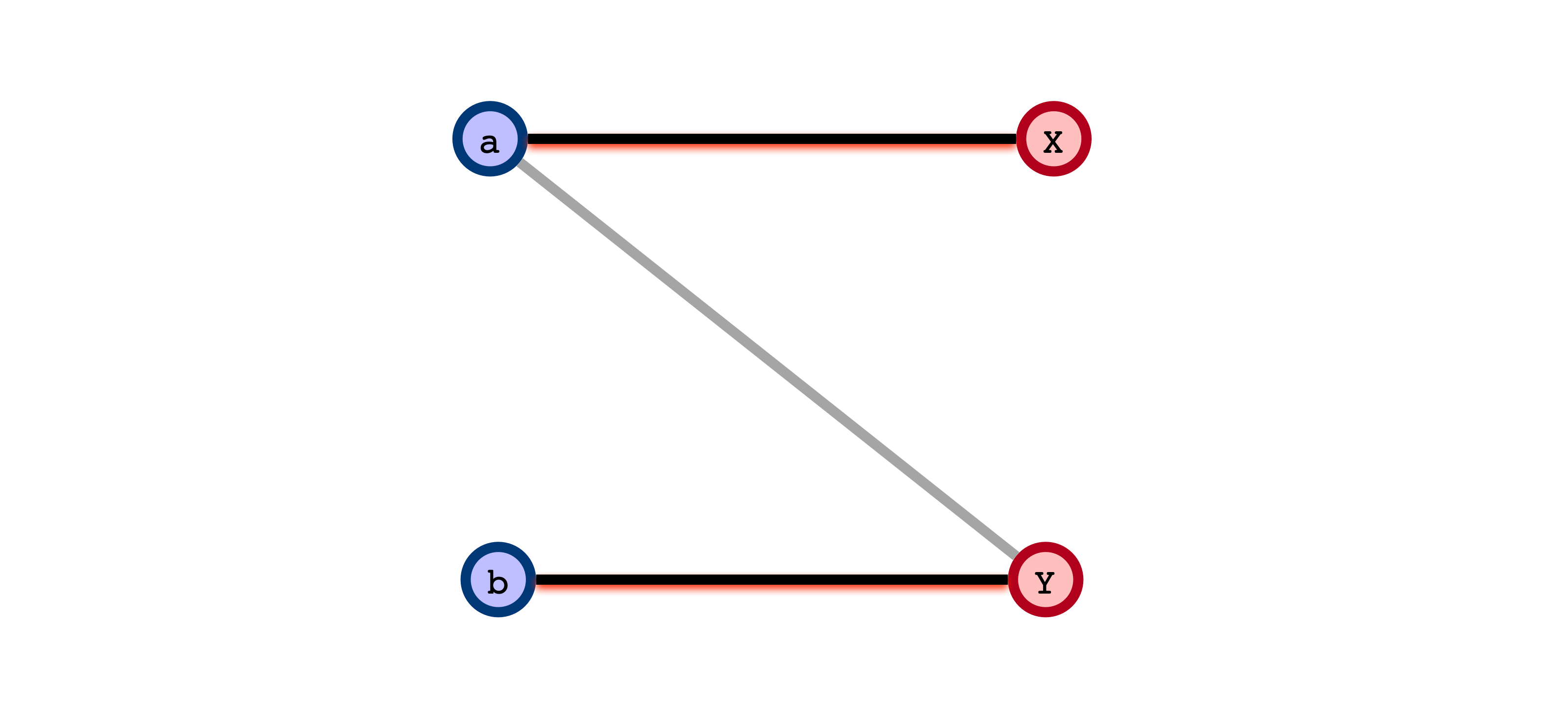
IV Form Matching from Flow
A Technicality
Assume all flows are integral flows:
- amount of flow across each edge is an integer
Note. Ford-Fulkerson always gives an integral flow.
Claim 1
If $G$ has a matching of size $k$, then $G’$ admits a flow $f$ of value $k$.
Claim 2
If $G’$ admits an integral flow of value $k$, then $G$ has a matching of size $k$.
Implications
- Value of the maximum flow in $G’$ equals the size maximum matching in $G$.
- Given a maximum (integral) flow in $G’$, we can find a maximum matching in $G$
Conclusions
- Found a reduction from Maximum Bipartite Matching to Max Flow
- Any (integral) Max Flow algorithm can be used to solve MBM
- any improvement in Max Flow algorithms will yield a corresponding improvement in MBM solution
- We showed MBM $\leq_P$ Max Flow
- MBM is “no harder” than Max Flow
- Max Flow is “no easier” than MBM
Next Time
Another view of $\leq_P$:
- suppose $A$ is a “hard” problem
- we show $A \leq_P B$
- then we’ve established that $B$ is no easier than $A$
- any efficient solution to $B$ would imply an efficient solution to $A$