Lecture 27: Shortest Paths, Revisited

$ \def\opt{ {\mathrm{opt}} } $

COSC 311 Algorithms, Fall 2022

Announcements

1. HW 05 Due this Friday
2. Midterm 2 Wednesday 11/16
   • in class
   • focus on material since last midterm up to this Friday
   • algorithmic paradigms:
     • divide and conquer
     • greedy
     • dynamic programming
     • network flow
   • mixture of computational and algorithm design questions
   • details forthcoming

Directed Graphs and Paths

Representing Directed Graphs

Adjacency List

• $v$’s neighbors are outgoing neighbors

Single Source Shortest Paths

Input:

• (Directed) graph $G = (V, E)$, edge weights $w$
• Starting vertex $u$

Output:

• $d(v) = $ distance from $u$ to $v$ for every vertex $v$
  • distance is length of shortest directed path from $u$ to $v$
  • length is sum of edge weights of path

Previous Algorithms

1. Breadth-first Search (BFS)
   • solves SSSP when all edge weights are $1$
2. Dijkstra’s Algorithm
   • solves SSSP when all edge weights are $\geq 0$

Example 1

Question 1. Why can Dijkstra fail when edge weights can be negative?

Example 2

Question 2. Why might shortest paths not exist when edge weights can be negative?

Assumption

Assume. $G$ does not contain any negative weight cycles.

Shortest Paths Again

Suppose shortest path from $u$ to $x$ contains $j$ hops.

• $v$ is $x$’s “parent” along path
• $d(u, x) = d(u, v) + w(v, x)$
• shortest path from $u$ to $v$ has $j-1$ hops

Dynamic Programming Approach

Idea. For each vertex $v$ and each $j = 1, 2, \ldots, n-1$ compute $d_j(u, v) = $ length of shortest path from $u$ to $v$ with at most $j$ hops.

• Note $d(u, v) = d_{n-1}(u, v)$.

Questions

Question 1. How to initialize $d_0(u, v)$?

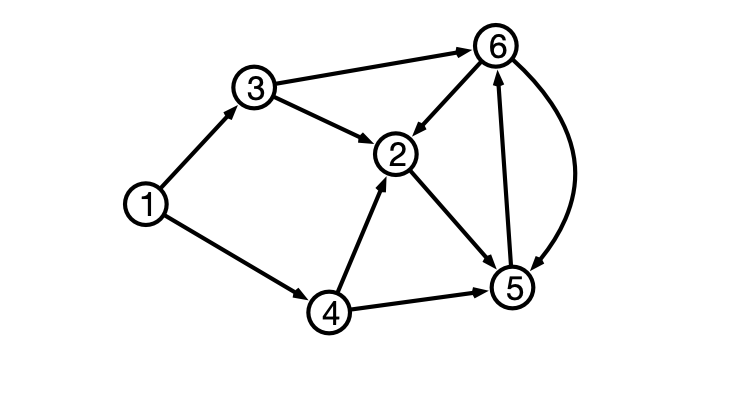
Illustration

Bellman-Ford Algorithm

  Bellman-Ford(V, E, w, u)
    d <- 2d array [0..n-1, 1..n]
    for v = 1 to n do d[0, v] <- infinity
    d[0, u] <- 0
    for j = 1 to n-1 do
      for each vertex v in V set d[j, v] <- d[j-1,v]
      for each vertex v in V
        for each neighbor x of v
          d[j, x] <- Min(d[j, x], d[j-1, v] + w[v, x])
    return d[n-1]

Running time?

Correctness

Claim. For all $j = 0, 1, \ldots, n-1$ and for all vertices $v$, $d[j, v]$ stores length of shortest path from $u$ to $v$ with $j$ or fewer hops. I.e., $d[j, v] = d_j(v)$

Proof. Induction on $j$.

Base case, $j = 0$.

Inductive Step, $j-1 \implies j$

• suppose $d[j-1, v] = d_{j-1}(v)$ for all $v$
• consider shortest path $P$ of $j$ hops from $u$ to $v$
• let $x$ be penultimate vertex in $P$
• then $d_j(v) = d_{j-1}(x) + w(x, v)$
• by inductive hypothesis, $d_{j-1}(x) = d[j-1,x]$
• therefore in iteration $j$, get $d[j, v] \leq d[j-1,x] + w(x, v) = d_{j-1}(x) + w(x, v) = d_j(v)$
• also have $d[j, v] \geq d_j(v)$ (why?)
• so $d[j, v] = d_j(v)$

Conclusion

If $G$ has no negative weight cycles, then Bellman-Ford solves single source shortest paths in $O(m n)$ time.

Dijkstra vs Bellman-Ford?

Running times:

• Dijkstra: $O(m \log n)$
• Bellman-Ford: $O(m n)$

Why pick Bellman-Ford over Dijkstra?

Bellman-Ford Again

  Bellman-Ford(V, E, w, u)
    d <- 2d array [0..n-1, 1..n]
    for v = 1 to n do d[0, v] <- infinity
    d[0, u] <- 0
    for j = 1 to n-1 do
      for each vertex v in V set d[j, v] <- d[j-1,v]
      for each vertex v in V
        for each neighbor x of v
          d[j, x] <- Min(d[j, x], d[j-1, v] + w[v, x])
    return d[n-1]

Next Time: Cold War

Rail Network of Eastern Europe

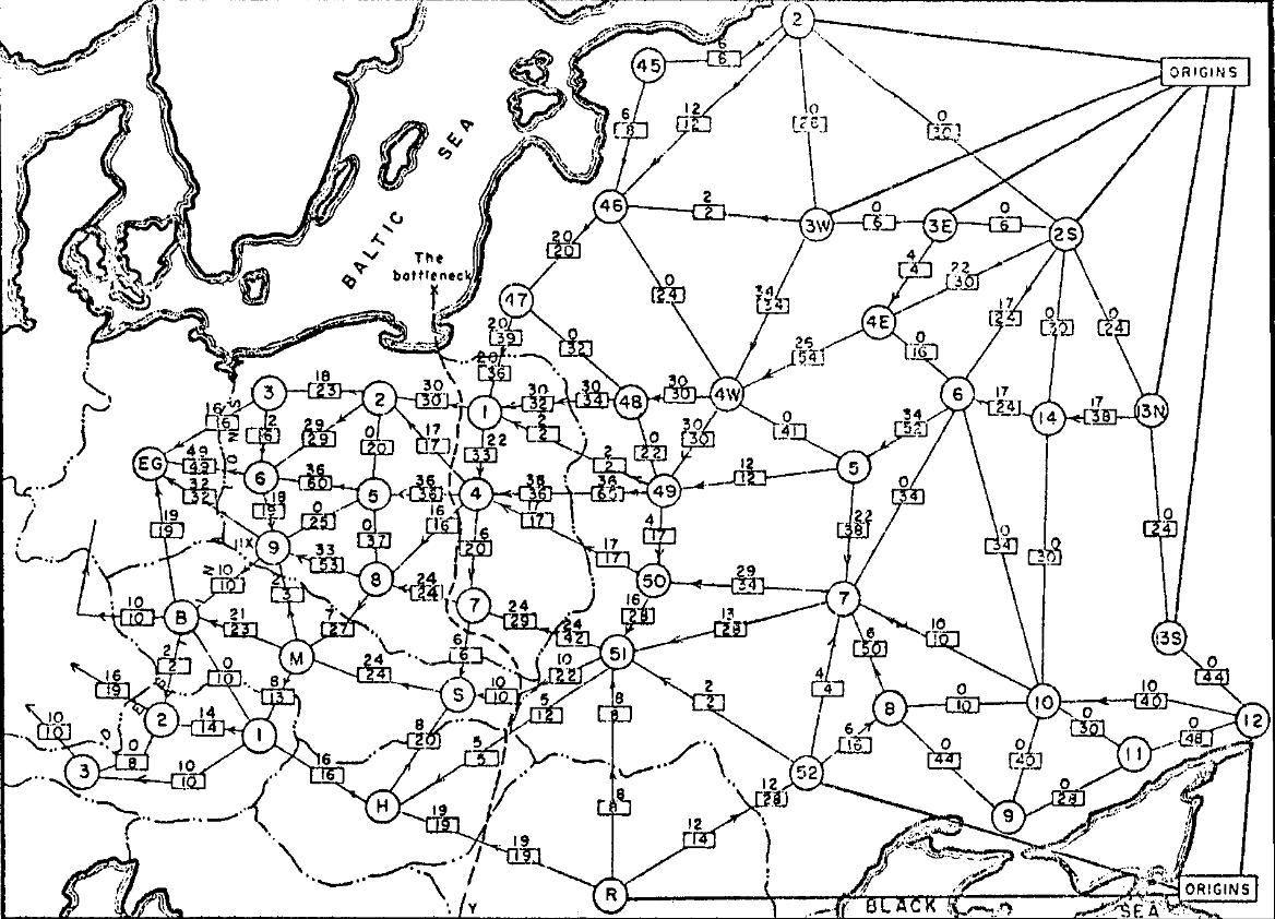
Networks to Graphs

Modeling the network:

• nodes represent railway junctions
• edges represent rail lines
• weights represent capacities of lines
  • capacity indicates tonnage that can cross line per unit time
  • proportional to cost of disrupting movement along line

Question 1. How much material can the USSR transport to Western Europe per unit time?

Question 2. What is the cheapest way to disrupt flow of material?

Network Flow

A new interpretation of directed graphs:

• network of (directional) pipes
• weights are capacities
  • how much fluid can flow through piper per time
• designated source node $s$
  • all edges directed away from $s$
• designated sink or destination node $t$
  • all edges directed towards $t$

Question. How much fluid be routed from $s$ to $t$ per unit time?