Lecture 16: Dijkstra’s Algorithm

COSC 311 Algorithms, Fall 2022

$ \def\compare{ {\mathrm{compare}} } \def\swap{ {\mathrm{swap}} } \def\sort{ {\mathrm{sort}} } \def\insert{ {\mathrm{insert}} } \def\true{ {\mathrm{true}} } \def\false{ {\mathrm{false}} } \def\BubbleSort{ {\mathrm{BubbleSort}} } \def\SelectionSort{ {\mathrm{SelectionSort}} } \def\Merge{ {\mathrm{Merge}} } \def\MergeSort{ {\mathrm{MergeSort}} } \def\QuickSort{ {\mathrm{QuickSort}} } \def\Split{ {\mathrm{Split}} } \def\Multiply{ {\mathrm{Multiply}} } \def\Add{ {\mathrm{Add}} } \def\cur{ {\mathrm{cur}} } \def\gets{ {\leftarrow} } $

Overview

1. Recap of DFS
2. Weighted Graphs
3. Weighted Shortest Paths
4. Dijkstra’s Algorithm

Last Time

Unweighted Single-Source Shortest Paths:

• Given graph $G = (V, E)$ and starting vertex $u$
• Find for every vertex $v$, the distance $d(u, v)$
  • $d(u, v) =$ length of shortest path from $u$ to $v$
  • shortest $= $ fewest hops

BFS Pseudocode

  BFS(V, E, u):
    intialize d[v] <- -1 for all v
    d[u] <- 0
    queue.add(u)
    while queue is not empty do
      v <- queue.remove()
      for each neighbor w of v do
        if d[w] = -1 then
          d[w] <- d[v] + 1
          queue.add(w)
    return d

Correctness. Follows from interaction with queue: vertices added in order of increasing distance from $u$

• $\implies$ distance is correct when vertex added

BFS Phases

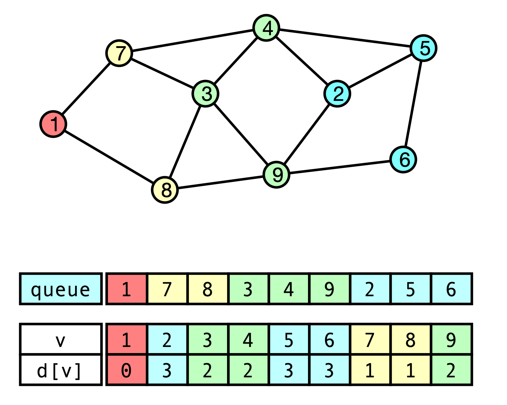
BFS Running Time?

  BFS(V, E, u):
    intialize d[v] <- -1 for all v
    d[u] <- 0
    queue.add(u)
    while queue is not empty do
      v <- queue.remove()
      for each neighbor w of v do
        if d[w] = -1 then
          d[w] <- d[v] + 1
          queue.add(w)
    return d

More General Problem

Definition. A weighted graph is a graph $G(V, E)$ where each edge $e \in E$ is additionally assigned a (real valued) weight $w(e)$.

• for now, assume $w(e) \geq 0$

Distance in Weighted Graphs

• $G = (V, E)$ a graph, $w$ weights

• $P = v_0 e_1 v_1 e_2 v_2 \cdots e_k v_k$ a path

• The (weighted) length of $P$ is

  \[w(P) = w(e_1) + w(e_2) + \cdots + w(e_k)\]

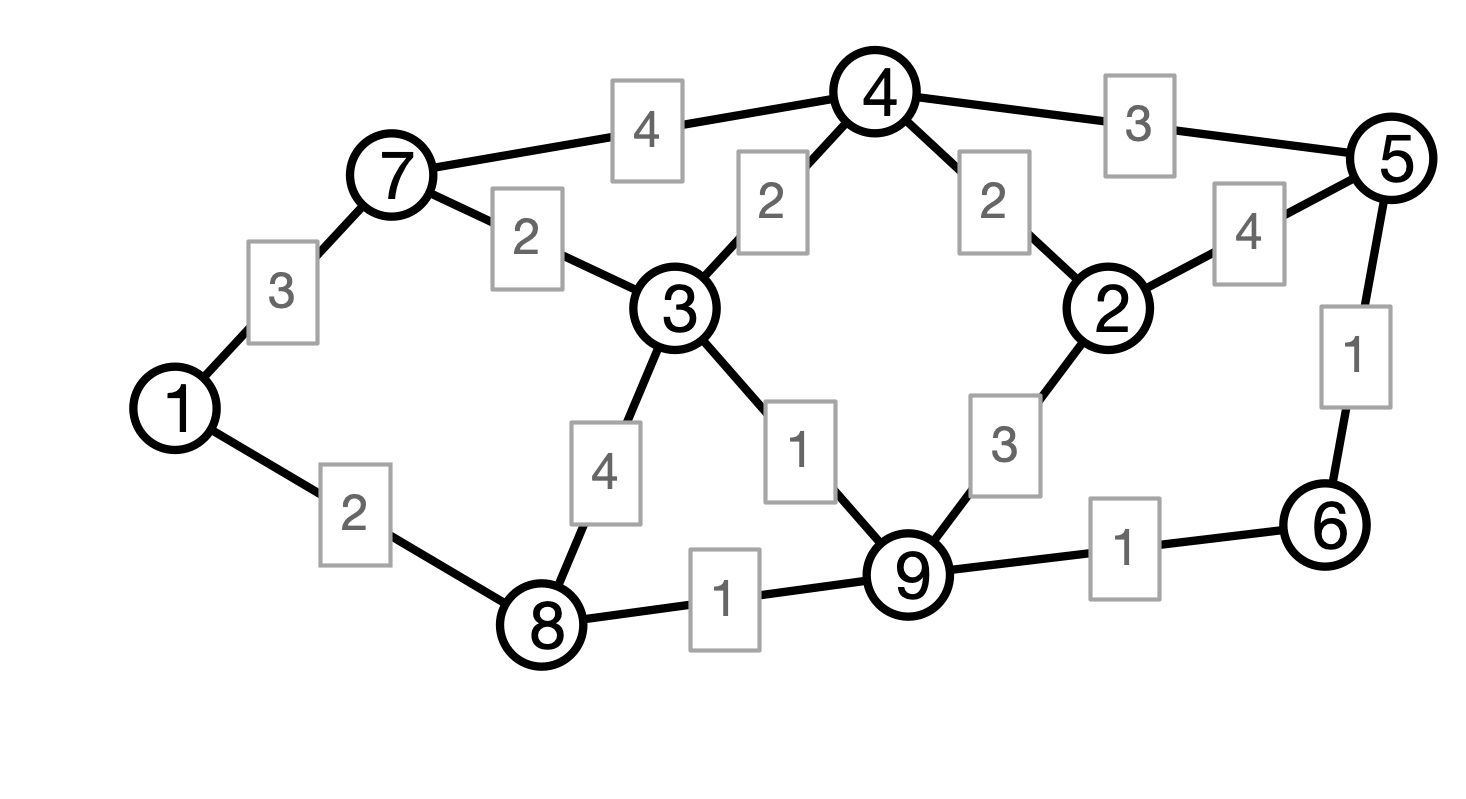
Example

Weighted Shortest Paths

Given weights $w$, define $d_w(u, v)$ to be minimum (weighted) length of any path $P$ from $u$ to $v$.

Example

What is $d_w(1, 3)$? What about $d_w(1, 5)$?

Weighted SSSP

Input.

• a weighted Graph $G = (V, E)$, edge weights $w$
• an initial vertex $u \in V$
• each vertex $v \in V$ has associated adjacency list
  • list of $v$’s neighbors
  • includes weight of edge from $v$ to each neighbor

Output.

• A map $d: V \to \mathbf{R}$ such that $d[v] = d_w(u, v)$ is the graph distance from $u$ to $v$

  • $d[v] = \infty$ indicates no path from $u$ to $v$

Weighted SSSP

Does BFS compute weighted distances from $u$?

• must update procedure
• when processing edge $(v, x)$, should update $d[x] \gets d[v] + w(v, x)$ rather than setting $d[x] \gets d[v] + 1$

Does this work?

Weighted BFS Example

Issue

• BFS processes vertices in order of fewest hops from $u$
• With weighted graphs, shortest path need not have fewest hops

BFS Analysis Takeaway

• BFS succeeds on unweighted graphs because closer vertices are processed before farther vertices

• Could we get similar behavior for weighted distances?

  • must ensure: vertices processed in order of weighted distance from $u$

  • how can we do this?

Dijkstra’s Algorithm

Idea. Process elements in order of weighted distance from $u$

• Maintain set $S$ of nodes whose distances from $u$ is known
• Find element $x \in V - S$ that is closest to $u$ and add it to $S$

Dijkstra’s Algorithm in Detail

1. Initialize $d[u] = 0$ and $d[v] = \infty$ for all $v \neq u$
2. Maintain set $S$ of finalized nodes, initially empty
3. Process nodes. While $S \neq V$ do:
   • find node $v$ in $V - S$ with minimal $d[v]$
   • add $v$ to $S$
   • for each neighbor $x$ of $v$
     • update $d[x] \gets \min (d[x], d[v] + w(v, x))$

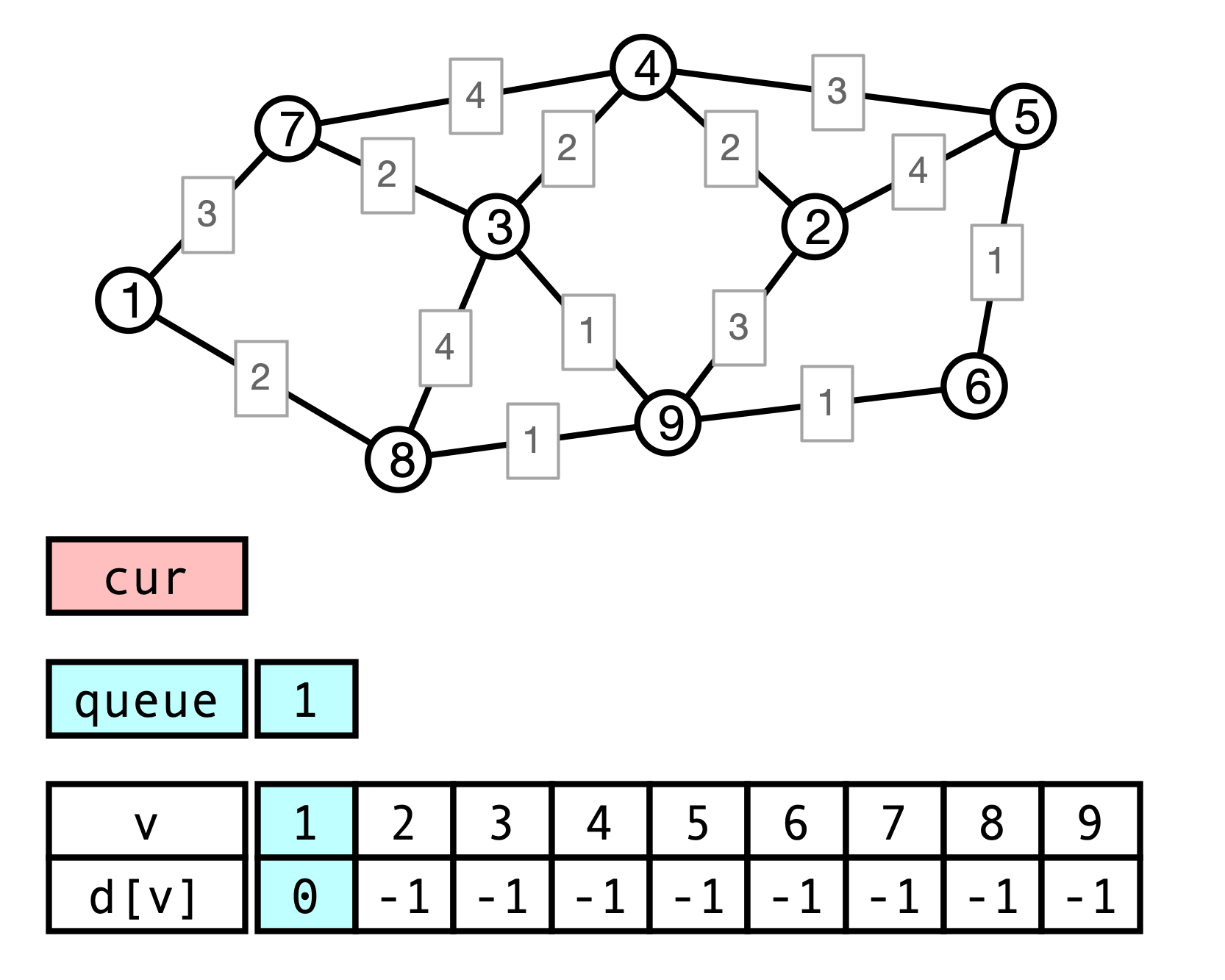
Dijkstra Illustration

Correctness

1. Initialize $d[u] \gets 0$ and $d[v] \gets \infty$ for all $v \neq u$
2. Maintain set $S$ of finalized nodes, initially empty
3. Process nodes: while $S \neq V$
   • find node $v$ in $V - S$ with minimal $d[v]$
   • add $v$ to $S$
   • for each neighbor $x$ of $v$
     • update $d[x] \gets \min (d[x], d[v] + w(v, x))$

Claim. For every vertex $v \in S$, $d[v]$ stores the correct (weighted) distance $d_w(u, v)$.

Proof of Claim

Claim. For every vertex $v \in S$, $d[v]$ stores the correct (weighted) distance $d_w(u, v)$.

Proof. Use induction on size of $S$. Set $k = $ size of $S$.

Base case $k = 1$. Only $u$ is added to $S$. Set $d[u] \gets 0$, which is correct answer.

Inductive Step I

Inductive hypothesis. When $S$ contains $k$ elements, $d[v]$ is correct for all vertices $v \in S$.

Consider next iteration of outer loop:

• $x$ has $d[x] = \min_{v \in S} (d[v] + w(v, x))$

Inductive Step II

Must show: $d[x] = d_w(u, x)$; argue by contradiction

1. suppose $d[x] \neq d_w(u, x)$
2. observe: there is a path from $u$ to $x$ of length $d[x]$
3. $\implies d_w(u, x) < d[x]$
4. $\implies$ there is a path $P$ from $u$ to $x$ of length $\ell < d[x]$

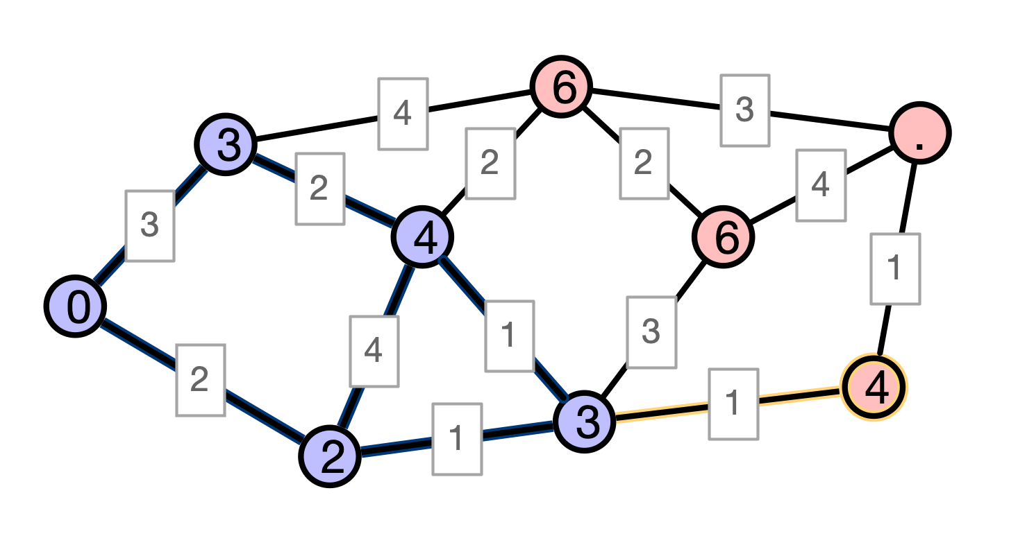
Shorter Path Illustration

Inductive Step III

Must show: $d[x] = d_w(u, x)$; argue by contradiction

1. suppose $d[x] \neq d_w(u, x)$
2. observe: there is a path from $u$ to $x$ of length $d[x]$
3. $\implies d_w(u, x) < d[x]$
4. $\implies$ there is a path $P$ from $u$ to $x$ of length $\ell < d[x]$
5. $P$ must leave $S$ at some point $y$
6. by definition of $x$, any path from $u$ to $y$ must be longer than $d[x]$
7. $\implies w(P) \geq d[x]$, which contradicts $4$

Conclusion. $d[x] = d_w(u, x)$, as claimed.

Next Time

1. Implementing Dijkstra’s algorithm
   • how do we find $x$ with minimum $d[x]$ efficiently?
   • review heaps/priority queues
2. Minimum spanning tree problem